Ai
-

YOLOv2和YOLOv3
YOLOv2 回顾一下YOLOv1有哪些缺陷? 边界框训练时回归不稳定,导致定位误差大。 每个网格只能预测两个边界框且只能识别一类目标。 小目标检测效果差。 针对以上的问题,YOLOv2进行了改进,下面从检测机制优化、网络结构优化、训练策略优化3个维度进行。 检测机制优化 锚框(Anchor Box)机制 YOLOv1每个网格只会预测一个目标,因为每个网格预测的B个边界框的类别概率都是共享的,要是有多2个目标的中心都落在了一个网格中,那么有一个目标就没法预测了。怎么解决了? 让每个边界框都对应一个类别概率,这样就能做到每个网格可以预测多个目标了。 每个边界框训练是没有基准的,这样训练的时候就很不稳定。如果预先定义边界框,使训练的时候按照这些预定义的边界框作为基准进行训练调整。这里做个类比来理解,假设我们的目标坐标是(8,8),那么如果没有设置基准,从坐标(0,0)找到(8,8)就相对比较远,那假设我们从(6,6)这个基准开始找,那找到(8,8)的概率就大了。 上面预先定义的边界框就称为先验框(anchor Box),那么新的问题来了,这个anchor Box我们每个网格设置多少个?设置什么样的形状了?实际的数据集中Ground Truth(真实标签)边界框有些是长方形、有些是正方形。 YOLOv2使用了K均值聚类算法用于生成先验框(Anchor Boxes),其核心目标是从训练数据中自动学习边界框的尺寸和比例,替代人工预设的锚框,从而提升检测召回率与定位精度。YOLOv2通过聚类COCO数据集,得到5个先验框尺寸(如(0.25,0.33), (0.5,0.75)...),覆盖常见物体形状。 pw,ph是先验框anchor的宽高(根据K类均值聚类得来),tx,ty,tw,th模型预测的偏移量(训练得到)。所以通过pw,ph,tx,ty,tw,th就可以计算出实际要预测的框bx,by,bw,bh。模型最终预测出tx,ty,tw,th这四个值就可以计算出bx,by,bw,bh。 这里需要注意 YOLOv2中对tx,ty进行了sigmod归一化,防止训练初期,中心点数值极大训练不稳定。 YOLOv2预测边界框的宽和高初始值是基于先验框而来,是模型对每个锚框输出宽高缩放因子(t_w, t_h),通过聚类生成的先验框指数变换得到最终宽高。而YOLOv1是根据图像实际宽高缩放而来。 全卷积网络与先验框 YOLOv1最后阶段使用的是全连接层,使用全连接层不仅仅参数量大,同时会将先前的特征图包含的空间信息破坏,在YOLOv2中改成了全卷积结构。 可以看到输出也发生了变化YOLOv1的输出是7 x 7 x (1+4+1+4+20),而YOLOv2输出是13 x 13 x k x (1 + 4 + 20),这里的k是每个网格的先验框数量,一般为5。(1+4+20)分别是锚框的置信度、边界框坐标、类别概率,每个anchor先验框都对应一个(1+4+20),也就是说每个先验框可以检测一个目标,这样就解决了YOLOv1中每个网格只能检测一个目标的问题,YOLOv2中每个网格有5个先验框,就可以检测最多5个类别。 网络结构优化 加入批量归一化: YOLOv1中每层卷积都是由线性卷积+非线性激活函数组成,由于批量归一化得到越来越普遍的应用,并且效果较好,因此在YOLOv2每层卷积层都加入了批量归一化。所以卷积层就变成了线性卷积+归一化+非线性激活函数组成。 融合高分辨率特征图:YOLOv1输出的特征图是13 x 13 x 1024,分辨率越低丢失的特征就越多。为了解决这个问题,YOLOv2在第17层单独抽出一层26 x 26 x 512的特征图,然后通过特殊的降采样得到13 x 13 x 256的特征图,最后将这个13 x 13 x 256的特征图与前面13 x 13 x 1024的相加,这样达到提高特征信息保留。 多尺度训练 YOLOv2在训练上也做了进一步的优化,因为同一张图像,缩放到不同尺寸,不同尺寸包含的图像信息也不同。因此为了提高精度,引入了多尺度训练训练机制。 具体就是在训练网络时,对图像按照320、352、384、416、448、480、512、544、576、608等不同输入尺寸进行训练。 总结一下,YOLOv2针对YOLOv1的改进点有以下。 增加先验框机制:每个网格使用K类均值聚类预设K个先验框作为基准训练。每个先验框负责预测一个目标。 加入批量归一化:每个卷积层对训练数据做批量归一化处理。 高分辨率特征图:网格划分13 x 13,主干网络中抽离一路高分辨率特征图进行特殊处理然后再加回去。 对尺度训练:训练阶段使用不同尺度的图像数据进行训练。 YOLOv3 对应目标检测网络可以由主干网络、颈部网络、检测头。 主干网络:提取多尺度特征。通过卷积层、池化层等操作,将输入图像逐层抽象化,生成不同层级的特征图。有浅层特征和深层特征。浅层特征是保留细节(如边缘、纹理),适合小目标检测;深层特征是蕴含语义信息(如物体整体结构),适合大目标识别。 颈部网络:融合与优化特征。连接主干网络与检测头,整合不同层级的特征图,增强模型对不同尺度目标的感知能力。 检测头:执行具体检测任务。基于融合后的特征,输出目标的位置、类别及置信度。 YOLOv2对于小目标的检测还是不够精确,这一缺陷的主要原因是YOLOv2只使用了32倍的降采样率。 浅层卷积层:没有经过更多的卷积层处理,提出的语义信息较少,具有较浅的语义信息;但对应没有过多的降采样因此具备较多的位置信息。 深层卷积层:经过更多的卷积层处理,提取更多的语义信息;但是位置信息经过了太多的降采样,丢失了位置信息。 语义信息可以理解为是什么类别的物品,位置信息是这个物品在图中的什么坐标位置。浅层卷积层更适合检测小目标(语义信息不需要这么多),深层卷积层适合检测大目标(需要更多的语义信息)。根据这个认知,YOLOv3主干网络就使用了3个不同尺寸的特征图,分布对应的降采样是32、16、8倍。对于小尺度目标使用的是8倍将采样并在浅层网络进行先提出输出针对性处理。而大尺度目标使用32倍降采样在最深层的网络中进行输出。 输入是416 x 416的图像,输出的是3个特征图,分布是C1=B X 256 X 52 X 52;C2=B x 512 x 26 x 26;C3=B x 1024 x 13 x 13,这里的B是先验框,一般为3。针对输入图像做了52x52、26x26、13x13三种不同疏密度的网格。 3个特征图根据多级检测结构推理后,得到最终预测的3个结果。y1= B x (4 + 1 + Nc) x 13 x 13;y2= B x (4 + 1 + Nc) x26 x 26;y3= B x (4 + 1 + Nc) x 52 x 52; 其中B为先验框数量,一般是3。Nc是类别个数,根据实际数据集,YOLOv3使用的是COCO数据集,有80个类别。 参考: 书籍《YOLO目标检测》 -

YOLOv1目标检测原理
介绍 YOLO在目标视觉检测应用广泛,You Only Look Once的简称。作者期望YOLO能像人一样只需要看一眼就能够立即识别其中的物体、位置及交互关系。能够达到快速、实时检测的效果。 YOLO检测系统可以简要分为3个步骤: Resize image:调整输入图像的大小为448 x 448。 Run Convolutional network:CNN卷积网络处理。 Non-max suppression:使用非极大值抑制。 YOLO与其他目标检测系统有什么不同或优势? YOLO 非常简单,如上图。单个卷积网络可以同时预测多个边界框及其类别概率。YOLO 使用完整图像进行训练,并直接优化检测性能。与传统的目标检测方法相比,这种统一的模型具有诸多优势。 首先,YOLO速度极快。由于YOLO将检测视为一个回归问题,因此无需复杂的流程。只需在测试时对一张新图像运行神经网络即可预测检测结果。 其次,YOLO在进行预测时会全局推理图像。与滑动窗口和基于区域提议的技术不同,YOLO在训练和测试期间会查看整幅图像,因此它隐式地编码了关于类别及其外观的上下文信息。Fast R-CNN 是一种领先的检测方法,由于无法看到更大的背景,它会将图像中的背景块误认为是物体。与 Fast R-CNN相比,YOLO 的背景错误率不到一半。 最后,YOLO学习的是可泛化的对象表征。在使用自然图像进行训练并在艺术作品上进行测试时,YOLO 的表现远超DPM和R-CNN 等领先的检测方法。由于 YOLO 具有高度的泛化能力,因此在应用于新领域或意外输入时,它不太可能崩溃。 更为详细的结构如下: 该网络包含24个卷积层和2个全连接层。不同于GoogLeNet使用的Inception模块,我们采用1×1降维层接3×3卷积层的简单设计。输入是448 x 448 x 3张量,最终输出是7×7×30的预测张量。 检测原理 YOLO是做统一检测,其网络使用整幅图像的特征来预测每个边界框。它还能同时预测图像所有类别的所有边界框。这意味着YOLO网络对整幅图像及其中的所有物体进行全局推理。 划分网格: 将输入图像划分为S X S个网格(grid)。 预测边界框:每个网格预测B个边界框(包含4个预测值x、y、w、h)并计算这些边界框的置信度分数以及C个条件类别概率。 置信度分数计算方式为:当网格中不存在任何物体,则为0,如果存在则等于预测框与真实框的交并比IOU。 C个条件类别概率:是C个预测类别,每个类别的概率值。因此总结一下,预测值为S X S X (B X 5 + C)个tensor。这里要注意的是,边界框的中心点并不是网格中心点,但中心点落在的这个网格负责这B个边界框的预测。 上面的图出之YOLOv1论文中的第5版本,如果不是很直观可以看看第1个版本,只不过第一个版本每个网格只预测一个边界框并且没有包含置信度。 为什么YOLOv1改进加了一个置信度? 预测框与真实框的交并比(定位质量),这样可以预测质量。YOLO将图像划分为网格,每个网格仅预测一组类别概率(与预测框数量无关),若直接用类别概率判断物体存在性,会忽略定位质量。例如一个网格预测出“狗”的概率为90%,但预测框可能严重偏离真实物体(IoU低),此时置信度会因低IoU而降低,避免高类别概率但定位差的误检。 为什么YOLOv1最开始每个网格是一个边界框后面变成了多个? 单框局限:每个网格仅预测一个边界框时,模型难以适应不同长宽比的物体(如瘦高的行人和扁平的汽车)。 多框设计:通过预测两个不同长宽比的边界框(如一个方形、一个长方形),模型可灵活匹配不同形状的目标,提高定位精度。 训练机制:训练时,选择与真实框IoU更高的预测框负责该物体,另一个框则被抑制(不参与损失计算),从而驱动网络学习多样化的边界框表达。 单框瓶颈:网格内若存在多个重叠目标(如密集人群),单框设计只能检测其中一个物体,导致漏检49。 冗余预测:两个边界框提供双重检测机会,即使一个框被错误抑制,另一框仍可能捕获未被覆盖的目标811。 但是这里需要注意的是,在YOLOv1中,同一个网格内的两个边界框(边界框1和边界框2)预测的类别结果是同一个类,因为类别的预测是共享的,也就是说预测的类别概率是共享的,每个网格只能预测一个类别目标。这也是YOLOv1的缺陷,如果有2个不同类别的物体中心都落在了同一个网格中,这样就没有同时预测两个物体。 总结:YOLO系统将检测建模为回归问题,它将图像划分为 S × S 的网格,并为每个网格单元预测 B 个边界框、这些框的置信度以及 C 个类别概率。这些预测被编码为S × S × (B ∗ 5 + C) 张量。为了在 PASCAL VOC 上评估 YOLO,作者使用 S = 7,B = 2。PASCAL VOC 有 20 个标记类别,因此 C = 20,最终预测是一个结果是7 × 7 × 30的张量。 损失函数 YOLOv1的损失函数使用的是边界框坐标(x,y,w,h)、置信度、类别概率计算而来,公式如下图。 边界框坐标损失:第一第二行公式,计算的是边界框坐标的损失。 置信度损失:分为有目标和无目标,无目标学习标签就是0,有目标学习标签是1. 类别损失:每个类别的损失,针对的是每个网格单元的损失,不是预测框的。 关于边界框的位置参数是怎么样的?下面总结一下: tx, ty: 是边界框中心坐标相对于当前网格(第5行第二列)左上角的偏移量(归一化到 [0,1] 区间)。 w, h: 是边界框的实际宽度和高度归一化到 [0,1],相对于整张图像的尺寸宽和高进行进行缩小比例。 详细的计算公式: 中心点坐标:x = (C_x + tx) / S, y = (C_y + ty) / S,(C_x, C_y为网格左上角坐标,S为网格划分数量) 宽高:w = 框宽 / 图宽, h = 框高 / 图高 YOLOv1的边界框参数优点是直接预测实际位置,无需先验框(Anchor Box),模型结构简单。缺点就宽高直接回归导致训练不稳定,定位精度较低; 模型后处理 YOLOv1模型训练完成后,给定一个448 x 448 x 3的tensor,模型输出是一个7 x 7 x 30的 tensor,也就是每个网格位置包含2个边界框的置信度输出C1和C2,两个边界框的位置参数(tx1,ty1,w1,h1)和(tx2,ty2,w2,h2)以及20个类别的概率p1~p20。 显然上面的输出结果不是我们想要的,我们要进行处理,筛选出最优的值,具体的处理步骤如下: 计算所有边界框得分:每个网格预测的边界框进行计算得分,计算公式分数=置信度值 x 类别概率中最大的值。 阈值剔除: 根据上一个步骤计算的得分,设定一个阈值比如0.3, 剔除小于阈值分数的边界框。 计算边界框位置:剔除一部分阈值后,计算编辑框的参数位置包括x,y,w,h。 非极大值抑制:经过前面的步骤后,同一个目标可能还是有多个预测边界框,最后试用非极大值抑制将重复检查的框去掉。最后就得到下面的示例结果。 总结一下YOLOv1的优缺点: 优点: 速度快,实时性强:首次实现端到端训练,推理速度达 45 FPS,简化了检测流程。 结构简单: 统一为单一回归问题,避免了区域提议(Region Proposal)的复杂步骤。 计算效率高:全卷积网络设计,适合资源受限的嵌入式设备。 缺点: 检测精度低:每个网格仅预测2个边界框且只能识别单一物体,同时对密集小目标检测效果差网络划分7x7精度不够。 定位不准确:边界框回归不稳定,导致定位误差大,与边界框的宽高定义为实际宽高缩放有关。 灵活性差:输入分辨率固定(448×448),不支持多尺度训练,网格划分(如 7×7)限制检测数量上限(最多 49 个物体)。 泛化能力弱:对非常规长宽比或重叠物体处理效果差。 参考: 1. 论文:https://arxiv.org/pdf/1506.02640v5 2. 书籍《YOLO目标检测》 -

opencv视频流
环境准备 本文通过采集USB摄像头来示例说明 export LD_LIBRARY_PATH=/mnt/extsd/usr/lib:$LD_LIBRARY_PATH #指定库的路径 cat /sys/devices/platform/soc/usbc0/usb_host #激活USB host 摄像头采集 摄像头相关的主要使用的是VideoCapture类。 打开摄像头 cv::VideoCapture cap; // 创建视频捕获对象 cap.open(0); // 打开默认摄像头(通常为/dev/video0) if (!cap.isOpened()) { std::cerr << "无法打开视频设备" << std::endl; return -1; } 设置参数 cap.set(cv::CAP_PROP_FRAME_WIDTH, 640); // 设置宽度 cap.set(cv::CAP_PROP_FRAME_HEIGHT, 480); // 设置高度 cap.set(cv::CAP_PROP_FPS, 30); // 设置帧率 采集数据 cv::Mat frame; while (true) { cap >> frame; // 捕获一帧 if (frame.empty()) { std::cerr << "捕获帧失败" << std::endl; continue; } // 在此处理帧数据... usleep(1000000 / frame_rate); // 30ms延迟,控制帧率 } 推流显示 主要是打开/dev/fb0,然后写入数据。 获取显示参数 通过ioctl的方式,获取显示分辨率,像素位深(每个像素的占用内存大小),以便将采集到的摄像头数据调整为合适的尺寸进行显示。 struct framebuffer_info get_framebuffer_info(const char* framebuffer_device_path) { struct framebuffer_info info; struct fb_var_screeninfo screen_info; int fd = -1; fd = open(framebuffer_device_path, O_RDWR); if (fd >= 0) { if (!ioctl(fd, FBIOGET_VSCREENINFO, &screen_info)) { info.xres_virtual = screen_info.xres_virtual; //虚拟水平的分辨率,包含不可见区域,即虚拟宽度 info.bits_per_pixel = screen_info.bits_per_pixel; //每个像素的位深,即像素大小,如16/24/32等 info.xres = screen_info.xres; //实际水平分辨率,即实际宽度 info.yres = screen_info.yres; //垂直分辨率,即实际高度 } } return info; }; 尺寸调整 cv::resize(frame, frame, cv::Size(fb_info.xres, fb_info.yres)); 从/dev/fb0获取的实际分辨率进行调整尺寸。 格式转换 写入前,先将采集的视频帧转换为屏幕显示支持的格式,如RGB565,RGBA等。 switch (framebuffer_depth) { case 16: //转换为RGB565格式输出 cv::cvtColor(frame, framebuffer_compat, cv::COLOR_BGR2BGR565); break; case 32: //转换为RGBA格式输出,添加一个alpha通道 std::vector<cv::Mat> split_bgr; cv::split(frame, split_bgr);//将BGR分离为3个通道,存储到split_bgr中。 split_bgr.push_back(cv::Mat(frame_size, CV_8UC1, cv::Scalar(255))); //创建一个全白的alpha通道矩阵并进行添加到一个新的通道 cv::merge(split_bgr, framebuffer_compat); //使用merge将3个颜色通道和alpha通道进行合并为RGBA四通道。 break; } 写入显示 ofs.seekp(0); //先进行定位 ofs.write(reinterpret_cast<char*>(framebuffer_compat.ptr(0)), framebuffer_compat.total() * framebuffer_compat.elemSize()); 也可以一行一行的写 for (int y = 0; y < frame_size.height; y++) { ofs.seekp(y * framebuffer_width * 2); ofs.write(reinterpret_cast<char*>(framebuffer_compat.ptr(y)), frame_size.width * 2); } 示例程序 #include <fcntl.h> #include <fstream> #include <iostream> #include <linux/fb.h> #include <signal.h> #include <stdint.h> #include <sys/ioctl.h> #include <unistd.h> #include <opencv2/opencv.hpp> static cv::VideoCapture cap; struct framebuffer_info { uint32_t bits_per_pixel; uint32_t xres_virtual; uint32_t xres; uint32_t yres; }; struct framebuffer_info get_framebuffer_info(const char* framebuffer_device_path) { struct framebuffer_info info; struct fb_var_screeninfo screen_info; int fd = -1; fd = open(framebuffer_device_path, O_RDWR); if (fd >= 0) { if (!ioctl(fd, FBIOGET_VSCREENINFO, &screen_info)) { info.xres_virtual = screen_info.xres_virtual; info.bits_per_pixel = screen_info.bits_per_pixel; info.xres = screen_info.xres; info.yres = screen_info.yres; } } return info; }; /* Signal handler */ static void terminate(int sig_no) { printf("Got signal %d, exiting ...\n", sig_no); cap.release(); exit(1); } int main(int, char**) { const int frame_width = 720; const int frame_height = 1280; const int frame_rate = 30; framebuffer_info fb_info = get_framebuffer_info("/dev/fb0"); std::cout << "xres virtua" << fb_info.xres_virtual << std::endl; std::cout << "bits per pixel" << fb_info.bits_per_pixel << std::endl; cap.open(0); if (!cap.isOpened()) { std::cerr << "Could not open video device." << std::endl; return 1; } std::cout << "Successfully opened video device." << std::endl; std::cout << "Display resolution:" << fb_info.xres << "x" << fb_info.yres << std::endl; cap.set(cv::CAP_PROP_FRAME_WIDTH, frame_width); cap.set(cv::CAP_PROP_FRAME_HEIGHT, frame_height); cap.set(cv::CAP_PROP_FPS, frame_rate); std::ofstream ofs("/dev/fb0"); cv::Mat frame; cv::Mat trams_temp_fream; cv::Mat yuv_frame; while (true) { cap >> frame; if (frame.depth() != CV_8U) { std::cerr << "Not 8 bits per pixel and channel." << std::endl; } else if (frame.channels() != 3) { std::cerr << "Not 3 channels." << std::endl; } else { //cv::transpose(frame, frame); //cv::flip(frame, frame, 0); cv::resize(frame, frame, cv::Size(fb_info.xres, fb_info.yres)); int framebuffer_width = fb_info.xres_virtual; int framebuffer_depth = fb_info.bits_per_pixel; cv::Size2f frame_size = frame.size(); cv::Mat framebuffer_compat; switch (framebuffer_depth) { case 16: cv::cvtColor(frame, framebuffer_compat, cv::COLOR_BGR2BGR565); break; case 32: std::vector<cv::Mat> split_bgr; cv::split(frame, split_bgr); split_bgr.push_back(cv::Mat(frame_size, CV_8UC1, cv::Scalar(255))); cv::merge(split_bgr, framebuffer_compat); break; } ofs.seekp(0); ofs.write(reinterpret_cast<char*>(framebuffer_compat.ptr(0)), framebuffer_compat.total() * framebuffer_compat.elemSize()); usleep(1000000 / frame_rate); } } } -

opencv图像处理
图像滤波 图像的滤波核心是使用一个小的矩阵(滤波器或卷积核)在图像上进行滑动卷积,将计算得到的结果作为目标像素的值。 均值滤波 cv::blur(InputArray src, OutputArray dst, Size ksize, Point anchor = Point(-1,-1), int borderType = BORDER_DEFAULT); src:输入的原始图像,支持Mat格式 dst:经过滤波处理的图像 ksize:滤波器大小,通常为2D大小,表示滤波的宽度和高度。 anchor:锚点指定窗口内的参考点,默认是Point(-1,-1)表示窗口中心点 boarderType:边界类型,用来处理边界参数的外推方式。 cv::Mat src = cv::imread("image.jpg", cv::IMREAD_GRAYSCALE); cv::Mat dst; cv::blur(src, dst, cv::Size(3, 3)); // 3x3的均值滤波 高斯滤波 void cv::GaussianBlur( const cv::Mat& src, cv::Mat& dst, cv::Size ksize, double sigmaX, double sigmaY = 0, int borderType = cv::BORDER_DEFAULT ); sigmaX:X方向的标准差,决定模糊的程度,值越大,模糊效果越强。 sigmaY:Y方向的标准差,默认是0,表示与X方向相同。 cv::GaussianBlur(src, dst, cv::Size(5, 5), 0); // 5x5的高斯滤波 中值滤波 void medianBlur(InputArray src, OutputArray dst, int ksize); ksize: 滤波器窗口大小 示例 cv::medianBlur(src, dst, 5); // 5x5的中值滤波 示例 下面示例,将图片使用高斯噪音处理,然后再使用滤波器进行模糊,噪音就可以看起来过滤掉。 #include <fcntl.h> #include <fstream> #include <iostream> #include <linux/fb.h> #include <signal.h> #include <stdint.h> #include <sys/ioctl.h> #include <unistd.h> #include <opencv2/opencv.hpp> using namespace cv; using namespace std; void add_gaussian_noise(Mat& image, double mean, double stddev) { Mat noise(image.size(), image.type()); randn(noise, mean, stddev); image = image + noise; } void display_image(const Mat& image, int framebuffer_width = 720) { static std::ofstream ofs("/dev/fb0"); cv::Mat framebuffer; cv::cvtColor(image, framebuffer, cv::COLOR_BGR2BGRA); cv::Size2f frame_size = framebuffer.size(); for (int y = 0; y < frame_size.height; y++) { ofs.seekp(y * framebuffer_width * 4); ofs.write(reinterpret_cast<char*>(framebuffer.ptr(y)), frame_size.width * 4); } } int main(int, char**) { Mat image = imread("test1.jpg", IMREAD_COLOR); if (image.empty()) { cerr << "Error: Could not open or find the image!" << endl; return -1; } double mean = 2.0; double stddev = 30.0; add_gaussian_noise(image, mean, stddev); display_image(image); cv::imwrite("noise.jpg", image); usleep(1000 * 1000 * 2); Mat dst; cv::GaussianBlur(image, dst, cv::Size(3, 3), 1); //cv::medianBlur(image, dst, 5); //cv::blur(src, dst, cv::Size(3, 3)); display_image(dst); cv::imwrite("dst.jpg", dst); } 如下图,中间是加了噪声的,最后一张是通过高斯滤波处理之后的。 图像形态学 膨胀与腐蚀 膨胀操作会增加图像中的白色区域或前景区域,使得图像中的对象或结构变得更大。具体来说,它会将图像中的每个像素点扩展到其邻域像素中(根据结构元素的大小和形状)。这意味着如果结构元素的一部分重叠在一个前景区域内,该区域就会被扩展。使白色区域扩展,物体变大。 cv2.dilate(src, dst=None, kernel, anchor=(-1, -1), iterations=1, borderType=cv2.BORDER_CONSTANT, borderValue=0) iteration:膨胀迭代次数,越大效果越明显 borderType:边界填充类型 borderValue:边界填充值,默认0是黑色 cv::Mat kernel = cv::getStructuringElement(cv::MORPH_RECT, cv::Size(3, 3)); //创建一个3*3的矩形结构元素 cv::dilate(src, dst, kernel); 腐蚀操作的效果与膨胀相反,它会减少图像中的白色区域或前景区域,使得图像中的对象变得更小。腐蚀操作会检查每个像素的邻域,如果邻域内的所有像素都是前景像素(白色),该像素才保持前景,否则变为背景(黑色)。使白色区域收缩,物体变小。 cv::Mat kernel = cv::getStructuringElement(cv::MORPH_RECT, cv::Size(3, 3)); cv::erode(src, dst, kernel); 以下是示例 #include <fcntl.h> #include <fstream> #include <iostream> #include <linux/fb.h> #include <signal.h> #include <stdint.h> #include <sys/ioctl.h> #include <unistd.h> #include <opencv2/opencv.hpp> void display_image(const cv::Mat& image, int framebuffer_width = 720) { static std::ofstream ofs("/dev/fb0"); if (!ofs) { std::cerr << "Error: Could not open framebuffer device!" << std::endl; return; } cv::Mat framebuffer; if (image.channels() == 1) { cv::cvtColor(image, framebuffer, cv::COLOR_GRAY2BGRA); } else if (image.channels() == 3) { cv::cvtColor(image, framebuffer, cv::COLOR_BGR2BGRA); } else if (image.channels() == 4) { image.copyTo(framebuffer); } else { std::cerr << "Error: Unsupported image format!" << std::endl; return; } cv::Size2f frame_size = framebuffer.size(); if (frame_size.width > framebuffer_width) { // 计算新的宽高,保持图像的纵横比 float aspect_ratio = frame_size.height / frame_size.width; int newWidth = framebuffer_width; int newHeight = static_cast<int>(newWidth * aspect_ratio); // 调整图像大小 cv::Mat resizedImage; cv::resize(framebuffer, resizedImage, cv::Size(newWidth, newHeight)); framebuffer = resizedImage; frame_size = resizedImage.size(); } for (int y = 0; y < frame_size.height; y++) { ofs.seekp(y * framebuffer_width * 4); ofs.write(reinterpret_cast<char*>(framebuffer.ptr(y)), frame_size.width * 4); } } int main(int, char**) { cv::Mat image = imread("test1.jpg", cv::IMREAD_COLOR); if (image.empty()) { std::cerr << "Error: Could not open or find the image!" << std::endl; return -1; } double mean = 2.0; double stddev = 30.0; display_image(image); usleep(1000 * 1000 * 1); cv::Mat dst; cv::Mat kernel = cv::getStructuringElement(cv::MORPH_RECT, cv::Size(5, 5)); cv::dilate(image, dst, kernel); display_image(dst); usleep(1000 * 1000 * 1); cv::erode(image, dst, kernel); display_image(dst); } 阈值化 阈值(Thresholding)是一种常见的图像分割方法,用于将灰度图像转换为二值图像。通过设置一个阈值,将像素值高于该阈值的区域设为白色(255),低于阈值的区域设为黑色(0),从而简化图像内容,便于后续处理。 二值化阈值:二值化是将图像中的像素值根据设定的阈值分为两类,通常用于简单的图像分割。 cv::threshold(src, dst, thresh, maxval, type); 示例:cv::threshold(src, dst, 127, 255, cv::THRESH_BINARY); thresh: 阈值,决定像素分类的分界线。 maxval:根据type选择,满足条件设置为最大值。 type: 阈值类型 自适应阈值:根据图像的局部区域动态计算阈值,适用于光照不均匀的图像。 cv::adaptiveThreshold( src, dst, maxValue, adaptiveMethod, thresholdType, blockSize, C); maxVaule:二值化的最大值,一般为255 adaptiveMethod: ADAPTIVE_THRESH_MEAN_C是使用邻域的均值作为阈值,ADAPTIVE_THRESH_GAUSSIAN_C :使用邻域的加权均值(高斯加权)作为阈值。 thresholdType:阈值类型,通常使用 THRESH_BINARY 或 THRESH_BINARY_INV。 blockSize:邻域的大小,必须是奇数(例如 3 , 5 , 7 , ...),该窗口在图像上滑动。 C:调整值,用于从计算的阈值中减去。调整结果的灵敏度。 cv::adaptiveThreshold(src, dst, 255, cv::ADAPTIVE_THRESH_MEAN_C, cv::THRESH_BINARY, 11, 2); 开闭运算、顶帽、黑帽 开运算:开运算是先进行腐蚀操作再进行膨胀操作。它通常用于去除小的噪点或小的物体,同时保留较大区域的结构。 闭运算:闭运算是先进行膨胀操作再进行腐蚀操作。它用于去除小的黑色区域(如小孔洞或空隙),并连接物体之间的细小裂缝。 顶帽:顶帽是开运算的结果与原图像之间的差异,主要用于提取比背景更亮的区域或小的亮点。 黑帽:黑帽是闭运算的结果与原图像之间的差异,主要用于提取比背景更暗的区域或小的暗点。 void cv::morphologyEx( InputArray src, OutputArray dst, int op, InputArray kernel, Point anchor = Point(-1, -1), int iterations = 1, int borderType = BORDER_CONSTANT, const Scalar&borderValue=morphologyDefaultBorderValue() ); kernel:结构元素,通常使用 cv::getStructuringElement() 生成。 op:形态学操作类型。 下面是op的类型 cv:MORPH_OPEN:开运算。 cv::MORPH_CLOSE:闭运算。 cv::MORPH_GRADIENT: 形态学梯度(膨胀 - 腐蚀),提取物体边缘。 cv::MORPH_TOPHAT :顶帽运算(原图 - 开运算结果),提取比背景亮的区域。 cv::MORPH_BLACKHAT 黑帽运算(闭运算结果 - 原图),提取比背景暗的区域。 示例 示例程序如下: int main(int, char**) { cv::Mat image = imread("test1.jpg", cv::IMREAD_GRAYSCALE); if (image.empty()) { std::cerr << "Error: Could not open or find the image!" << std::endl; return -1; } cv::Mat binary_img; cv::threshold(image, binary_img, 128, 255, cv::THRESH_BINARY); cv::Mat kernel = cv::getStructuringElement(cv::MORPH_RECT, cv::Size(5, 5)); cv::Mat dst; cv::Mat opened_img, closed_img, tophat_img, blackhat_img; cv::morphologyEx(binary_img, opened_img, cv::MORPH_OPEN, kernel); cv::morphologyEx(binary_img, closed_img, cv::MORPH_CLOSE, kernel); cv::morphologyEx(binary_img, tophat_img, cv::MORPH_TOPHAT, kernel); cv::morphologyEx(binary_img, blackhat_img, cv::MORPH_BLACKHAT, kernel); display_image(image); usleep(1000 * 1000 * 2); display_image(binary_img); usleep(1000 * 1000 * 2); display_image(closed_img); usleep(1000 * 1000 * 2); display_image(tophat_img); usleep(1000 * 1000 * 2); display_image(blackhat_img); } 图像边缘检测 canny Canny边缘检测是一个多阶段的图像处理算法,用于提取图像中的边缘。它的目标是识别图像中强度变化较大的区域,即边缘 int main(void) { cv::Mat image = cv::imread("test1.jpg", cv::IMREAD_GRAYSCALE); if (image.empty()) { std::cerr << "Error: Could not open image!" << std::endl; return -1; } // 进行 Canny 边缘检测 cv::Mat edges; cv::Canny(image, edges, 100, 200); // 低阈值 100,高阈值 200 display_image(edges); return 0; } 下面是处理的前后效果。 霍夫变换 霍夫变换(Hough Transform)是一种用于检测图像中的几何形状(如直线、圆等)的方法。它主要用于图像中的特征检测,特别是在噪声较大的图像中,可以有效地进行形状的识别。霍夫变换的基本思想是将图像中的边缘点通过一种数学映射,转化到参数空间,然后在参数空间中寻找对应的曲线(或直线、圆等)。 霍夫线变换: 检测线。 cv2.HoughLinesP(image, rho, theta, threshold, minLineLength, maxLineGap) image: 输入图像,通常是经过边缘检测(如 Canny 边缘检测)后的二值图像。 rho: 直线距离精度,单位是像素,通常设置为 1。 theta: 角度精度,单位是弧度,通常设置为 np.pi / 180(即 1°)。 threshold: 最小投票数,当某一候选直线在参数空间中的投票数大于此阈值时,认为检测到直线。 minLineLength: 最小直线长度。只有长度大于该值的直线才会被返回。 maxLineGap: 最大直线间隙。如果两段直线之间的间隙小于该值,则认为它们是同一条直线的两部分 int main(void) { cv::Mat img = cv::imread("test1.jpg"); if (img.empty()) { std::cerr << "Error: Could not open image!" << std::endl; return -1; } // 图像预处理:边缘检测 cv::Mat edges; cv::Canny(img, edges, 50, 150); // 使用 Canny 边缘检测 display_image(edges); usleep(1000 * 1000); // 使用 HoughLinesP 进行霍夫变换(概率霍夫变换) std::vector<cv::Vec4i> lines; cv::HoughLinesP(edges, lines, 1, CV_PI / 180, 50, 50, 10); // 参数为 (边缘图像, 输出的直线, ρ精度, θ精度, 阈值, 最小线段长度, 最大线段间隙) // 绘制检测到的直线 cv::Mat result = img.clone(); //cv::cvtColor(result, result, cv::COLOR_GRAY2BGR); // 将灰度图转为彩色图以显示彩色直线 for (size_t i = 0; i < lines.size(); i++) { cv::Vec4i l = lines[i]; cv::line(result, cv::Point(l[0], l[1]), cv::Point(l[2], l[3]), cv::Scalar(255, 0, 0), 2); // 绘制直线 } display_image(result); return 0; } 上面的示例中,先使用canny进行边缘处理,然后送入到霍夫变换中进行检测,最后绘制成直线。下面是检测后的效果。 霍夫圆变换: 检测圆。 cv2.HoughCircles(image, method, dp, minDist, param1, param2, minRadius, maxRadius) image: 输入图像,通常是灰度图像。 method: 霍夫变换的检测方法。对于 HoughCircles,一般使用 cv2.HOUGH_GRADIENT。 dp: 分辨率反比,表示霍夫空间的分辨率与图像分辨率的比例。通常设置为 1。 minDist: 设定圆心之间的最小距离,防止检测到相互靠得太近的圆。 param1: 边缘检测的高阈值(Canny 边缘检测的高阈值)。 param2: 圆的中心检测阈值,较小的值会检测到更多的圆,较大的值会检测较少的圆。 minRadius: 最小圆半径(单位:像素)。 maxRadius: 最大圆半径(单位:像素)。 int main(void) { cv::Mat img = cv::imread("test1.jpg"); if (img.empty()) { std::cerr << "Error: Could not open image!" << std::endl; return -1; } // 进行边缘检测 cv::Mat edges; cv::Canny(img, edges, 50, 150); display_image(edges); usleep(1000 * 1000); // 存储检测到的圆 std::vector<cv::Vec3f> circles; // 使用霍夫圆变换检测圆 cv::HoughCircles(edges, circles, cv::HOUGH_GRADIENT, 1, 23, 80, 52, 27, 100); // 在原图上绘制检测到的圆 cv::Mat result = img.clone(); for (size_t i = 0; i < circles.size(); i++) { cv::Point center(cvRound(circles[i][0]), cvRound(circles[i][1])); int radius = cvRound(circles[i][2]); // 绘制圆心 cv::circle(result, center, 3, cv::Scalar(0, 255, 0), -1); // 绘制圆 cv::circle(result, center, radius, cv::Scalar(255, 0, 0), 3); } display_image(result); return 0; } 同样是先使用canny检测进行处理,然后再使用霍夫圆进行检测圆,最后试用cv::circle进行绘制。 -

opencv基础操作
图像的读取和显示 读写图像 cv::Mat image = cv::imread("image.jpg", cv::IMREAD_COLOR); 使用imread函数读取图像,第一个参数是图像文件的路径,第二个参数是解释图像的颜色和格式(如彩色图像、灰度图像等)。第二个参数可省略,默认是cv::IMREAD_COLOR,以彩色图像读取。 cv::imwrite("output.jpg", image); 使用imwrite存储图像。 显示 使用imshow基于图像用户界面的显示方式,这种方式用于桌面的计算机,直接在屏幕上展示图像。 cv::imshow("Window title", image); cv::waitKey(0); // 等待按键按下 通过/dev/fb0节点写入,这种方式一般应用在嵌入式平台上,写入屏幕的驱动中。 std::ofstream ofs("/dev/fb0"); cv::Mat framebuffer; 定义一个存储图像像素数据的容器 cv::cvtColor(frame, framebuffer, cv::COLOR_BGR2BGR565); 将图像格式进行转换为与驱动支持的格式BGR565 ofs.write(reinterpret_cast<char*>(framebuffer.ptr(0)), framebuffer.total() * framebuffer.elemSize()); //现将framebuffer强制转换为char*格式,确保内存数据按字节进行处理。 //framebuffer.total()返回的是像素总元素数量,如果framebuffer是多通道,那就返回总数 //framebuffer.elemSize()返回的是每个像素字节大小。 //需要注意的是使用一次性写入,要注意fb的位置,每次写需要重新定位 还有另外一种写法,每一行每一行的刷新 cv::Size2f frame_size = frame.size(); cv::cvtColor(frame, framebuffer_compat, cv::COLOR_BGR2BGR565); for (int y = 0; y < frame_size.height; y++) { ofs.seekp(y * framebuffer_width * 2); //定位一行的位置,framebuffer_width是宽,即每行多少个像素 //*2是每个像素多少个字节,BGR565是2个字节。 ofs.write(reinterpret_cast<char*>(framebuffer_compat.ptr(y)), frame_size.width * 2); //写入一行数据,一行的数据量为frame_size.width * 2 } 下面是封装的示例函数 void display_image(const cv::Mat& image, int framebuffer_width = 720) { static std::ofstream ofs("/dev/fb0"); if (!ofs) { std::cerr << "Error: Could not open framebuffer device!" << std::endl; return; } cv::Mat framebuffer; if (image.channels() == 1) { cv::cvtColor(image, framebuffer, cv::COLOR_GRAY2BGRA); } else if (image.channels() == 3) { cv::cvtColor(image, framebuffer, cv::COLOR_BGR2BGRA); } else if (image.channels() == 4) { image.copyTo(framebuffer); } else { std::cerr << "Error: Unsupported image format!" << std::endl; return; } cv::Size2f frame_size = framebuffer.size(); if (frame_size.width > framebuffer_width) { // 计算新的宽高,保持图像的纵横比 float aspect_ratio = frame_size.height / frame_size.width; int newWidth = framebuffer_width; int newHeight = static_cast<int>(newWidth * aspect_ratio); // 调整图像大小 cv::Mat resizedImage; cv::resize(framebuffer, resizedImage, cv::Size(newWidth, newHeight)); framebuffer = resizedImage; frame_size = resizedImage.size(); } for (int y = 0; y < frame_size.height; y++) { ofs.seekp(y * framebuffer_width * 4); ofs.write(reinterpret_cast<char*>(framebuffer.ptr(y)), frame_size.width * 4); } } 示例 int main() { cv::Mat test_image = cv::imread("test.jpg"); if (test_image.empty()) { std::cerr << "Could not open the image" << std::endl; return -1; } std::ofstream ofs("/dev/fb0"); if (!ofs.is_open()) { std::cerr << "Failed to open framebuffer device." << std::endl; return -1; } // 将 BGR 图像转换为 BGRA 格式(RGB8888) cv::Mat framebuffer; cv::cvtColor(test_image, framebuffer, cv::COLOR_BGR2BGRA); ofs.write(reinterpret_cast<char*>(framebuffer.ptr(0)), framebuffer.total() * framebuffer.elemSize()); return 0; } 几何变换 这里的变换指的是缩放、旋转、平移、翻转。 裁剪与缩放 缩放 cv::Mat resizedImage; cv::resize(image, resizedImage, cv::Size(newWidth, newHeight)); 裁剪 Rect roi(100, 100, 200, 200); // (x, y, width, height) //先于x,y坐标开始,再按照width,height定义一个矩形框。 Mat croppedImage = image(roi); //将矩形框作用在image上,得到一个新的图像croppedImage 旋转 // cv::Point2f用于表示二维浮点坐标的类,下面是计算旋转中心点。 cv::Point2f center(image.cols / 2.0, image.rows / 2.0); // 用于计算二维旋转的仿射变换矩阵,45是旋转角度,1.0是缩放比例。 cv::Mat rotationMatrix = cv::getRotationMatrix2D(center, 45.0, 1.0); // 声明存储旋转后图像的变量 cv::Mat rotatedImage; // 执行仿射变换进行图像旋转 cv::warpAffine(image, rotatedImage, rotationMatrix, image.size()); 翻转 cv::Mat flippedImage; cv::flip(image, flippedImage, 1); // 1表示水平翻转,0表示垂直翻转 颜色变换 图像的颜色空间包括RGB、灰度和HSV等。 RGB:RGB是最常见的颜色空间,表示红、绿、蓝三个通道。 灰度:灰度图像只有一个通道,表示亮度。 HSV:HSV颜色空间表示色调(Hue)、饱和度(Saturation)和亮度(Value)。 颜色空间转换 RGB转灰度 cv::Mat grayImage; cv::cvtColor(image, grayImage, cv::COLOR_BGR2GRAY); RGB转HSV cv::Mat hsvImage; cv::cvtColor(image, hsvImage, cv::COLOR_BGR2HSV); RGB转RGB565 cv::Mat rgb565Image; cv::cvtColor(rgb565Image, framebuffer, cv::COLOR_BGR2BGR565); 通道分离 这里的通道指的是图像通道比如RGB的R/G/B 3个通道。通道分离的场景是分析每个颜色通道的像素值,比如在检测红色物体时,可以单独分析红色通道。另外还可以用做图像增强,对不同通道应用不同的增强算法,然后再合并。 通道分离 std::vector<cv::Mat> channels; //分离出的通道存储到channels中 cv::split(image, channels); 通道合并 cv::Mat mergedImage; cv::merge(channels, mergedImage); 示例代码 int main() { cv::Mat test_image = cv::imread("test.jpg"); if (test_image.empty()) { std::cerr << "Could not open the image" << std::endl; return -1; } double angle = 90; // 计算旋转中心点 cv::Point2f center(test_image.cols / 2.0, test_image.rows / 2.0); // 计算旋转矩阵 cv::Mat rotationMatrix = cv::getRotationMatrix2D(center, angle, 1.0); // 声明存储旋转后图像的变量 cv::Mat rotatedImage; // 执行仿射变换进行图像旋转 cv::warpAffine(test_image, rotatedImage, rotationMatrix, test_image.size()); std::ofstream ofs("/dev/fb0"); if (!ofs.is_open()) { std::cerr << "Failed to open framebuffer device." << std::endl; return -1; } // 将 BGR 图像转换为 BGRA 格式(RGB8888) cv::Mat framebuffer; cv::cvtColor(rotatedImage, framebuffer, cv::COLOR_BGR2BGRA); ofs.write(reinterpret_cast<char*>(framebuffer.ptr(0)), framebuffer.total() * framebuffer.elemSize()); return 0; } 总结 本章节总结opencv操作常用的数据结构。 Mat Mat对象的用途主要为存储图像、创建和操作多维矩阵。Mat数据类型分为两部分:信息头+指向像素数据的矩阵指针,信息头存储的是图像的尺寸、存储方法、存储地址。指向像素的矩阵指针为字面意思,即指向存储所有像素值的矩阵指针。 Mat A, C; //只创建信息头 A = imread(argv[1], IMREAD_COLOR); //为矩阵开辟内存空间。 Mat B(A); // Use the copy constructor C = A; // Assignment operator 如果在读取图像的时候只想获取图像中的部分图像(感兴趣的区域ROI),可以使用Rect和Range来标中数据。 Mat D (A, Rect(10, 10, 100, 100) ); // using a rectangle Mat E = A(Range::all(), Range(1,3)); // using row and column boundaries 其中Rect(10,10,100,100)前两位是坐标,后两位指定宽高,示例如下。 Range::all()选中所有的行,Range(1,3)选中1~3列。 Mat对象作为通用矩阵类和图像容器,容器中存储的是原始的像素值。在opencv中描述这些像素值有专门的数据格式。 Mat Img(640, 640, CV_8UC3); 上述中640*640大小的图像,存储的数据类型是CV_U8C3,这里的CV_U8C3格式为基本数据类型+通道数。"CV_"表示前缀,"8"表示每个像素值的位深比特数,有8/16/32/64bits,"U"表示数据类型为无符号,"C3"表示通道数RGB。关于通道一般有几种,示例如下: 1通道:灰度图像 3通道:RGB通道,图像由红、绿、蓝三色组成。 4通道:在RGB通道基础上,加一个透明通道。 Scalar Scalar用于表示颜色或像素的值,他是一个模板类,存储了4个值,每个值代表图像的颜色通道,如BGR或HSV。 template<typename _Tp> class Scalar_ { public: _Tp val[4]; // 颜色值,最多支持四个通道 .... }; cv::Scalar(0, 0, 255); // 红色 BGR 颜色,表示 (蓝色 = 0, 绿色 = 0, 红色 = 255) cv::Scalar(255, 0, 0); // 蓝色 BGR 颜色,表示 (蓝色 = 255, 绿色 = 0, 红色 = 0) cv::Scalar(0, 255, 0); // 绿色 BGR 颜色,表示 (蓝色 = 0, 绿色 = 255, 红色 = 0) cv::Scalar(0, 255, 0, 128); // 半透明绿色 cv::Scalar(255, 0, 0, 255); // 完全不透明的蓝色 Size Size类用来表示图像的大小、矩阵的尺寸。 class Size { public: Size(); Size(int _width, int _height); Size(double _width, double _height); int width; // 图像宽度 int height; // 图像高度 }; 下面是常用的用法。 设置图像的尺寸 cv::Mat image = cv::imread("image.jpg"); cv::Size new_size(800, 600); // 新的尺寸 cv::resize(image, image, new_size); // 将图像调整为新尺寸 获取图像的尺寸 cv::Mat image = cv::imread("image.jpg"); cv::Size image_size = image.size(); // 获取图像尺寸 创建一个尺寸大小的矩阵 cv::Mat mat(cv::Size(400, 300), CV_8UC1); // 创建一个大小为 400x300 的单通道图像 cvtColor cvtColor用于颜色空间的转化,图像的颜色空间一般有RGB,BGR(RGB存储顺序的不同),HSV,Lab等,其可以将图像从一种颜色空间变换为另一种颜色空间。 cv::Mat cv::cvtColor(const cv::Mat& src, cv::Mat& dst, int code, int dstCn = 0); src: 输入图像 dst:输出图像 code:指定转化格式,如 cv::COLOR_BGR2GRAY,cv::COLOR_BGR2HSV。 dstCn:输出通道数,如果是0,表示通道数与目标颜色空间通道匹配。 RGB转BGR cv::Mat src = cv::imread("image.jpg"); // 读取 RGB 图像(如果图像是 RGB 格式的话) cv::Mat bgr; cv::cvtColor(src, bgr, cv::COLOR_RGB2BGR); // 转换为 BGR 图像 HSB转BRG cv::Mat hsv = cv::imread("image_hsv.jpg"); // 读取 HSV 图像 cv::Mat bgr; cv::cvtColor(hsv, bgr, cv::COLOR_HSV2BGR); // 转换为 BGR 图像 BRG转灰度 cv::Mat src = cv::imread("image.jpg"); // 读取 BGR 图像 cv::Mat gray; cv::cvtColor(src, gray, cv::COLOR_BGR2GRAY); // 转换为灰度图 -

优化算法
局部最小与全局最小 对应任何目标函数f(x),当然这里的目标函数可以是损失函数。如果在x处对应的f(x)小于x附近任意点的f(x),那么f(x)是局部最小的。如果f(x)在x处的值是整个域中目标函数的最小值,那么f(x)是全局最小值。 除了局部最优解外,鞍点也是梯度为0的区域。什么是鞍点了?如下图。 在深度学习模型训练中,通常往往会有许多局部最优解或鞍点,要解决这种局部最优解需要一定程度的噪音才能使参数跳出局部最小值,实际上使用小批量随机梯度下降也可以将参数从局部极小值中跳出。 梯度下降(gd) 对于多变量的输入$\mathbf{x} = [x_1, x_2, \ldots, x_d]^\top$的情况。它的梯度也是多元的,是一个由$d$个偏导数组成的向量: $$\nabla f(\mathbf{x}) = \bigg[\frac{\partial f(\mathbf{x})}{\partial x_1}, \frac{\partial f(\mathbf{x})}{\partial x_2}, \ldots, \frac{\partial f(\mathbf{x})}{\partial x_d}\bigg]^\top$$ 梯度中的每个偏导数元素$\partial f(\mathbf{x})/\partial x_i$代表了当输入$x_i$时$f$在$\mathbf{x}$处的变化率。最陡下降的方向由负梯度$-\nabla f(\mathbf{x})$得出。选择合适的学习率$\eta > 0$来生成典型的梯度下降算法: $$\mathbf{x} \leftarrow \mathbf{x} - \eta \nabla f(\mathbf{x})$$ 假设一个目标函数$f(\mathbf{x})=x_1^2+2x_2^2$,并有二维向量$\mathbf{x} = [x_1, x_2]^\top$作为输入,标量作为输出。则梯度$\nabla f(\mathbf{x}) = [2x_1, 4x_2]^\top$给出。下面是梯度从[-5,-2]开始进行下降。 注意,在实际训练时,如果f(x)是损失函数,那么x就是参数,通常对应的是w。 随机梯度下降(sgd) 在深度学习中,在训练数据时,有很多样本,按照前面的梯度下降方法,那么对于多个样本的损失我们可以使用平均值来表示。给定$n$个样本的训练数据集,我们假设$f_i(\mathbf{w})$是关于索引$i$的训练样本的损失函数,其中$\mathbf{w}$是参数向量,我们得到损失函数为: $$f(\mathbf{w}) = \frac{1}{n} \sum_{i = 1}^n f_i(\mathbf{w})$$ $\mathbf{w}$的目标函数的梯度计算为 $$\nabla f(\mathbf{w}) = \frac{1}{n} \sum_{i = 1}^n \nabla f_i(\mathbf{w})$$ 如果使用梯度下降法,每计算一次梯度,需要对所有的样本做计算求平均,如果每个自变量迭代的计算代价为$\mathcal{O}(n)$,它随$n$线性增长。这样的方法虽然计算梯度准确性高,但是当训练数据集较大时,每次迭代的梯度下降计算代价将较高。 随机梯度下降(SGD)就是要降低计算量,在计算梯度时,不要对所有样本进行计算,而是在随机梯度下降的每次迭代中,对数据样本随机均匀采样一个索引$i$,也就是只取一个样本计算计算梯度, 其中$i\in{1,\ldots, n}$,并计算梯度$\nabla f_i(\mathbf{w})$以更新$\mathbf{w}$: $$\mathbf{w} \leftarrow \mathbf{w} - \eta \nabla f_i(\mathbf{w}),$$ 其中$\eta$是学习率。可以看到,每次迭代的计算代价从梯度下降的$\mathcal{O}(n)$降至常数$\mathcal{O}(1)$。此外,我们要强调,随机梯度$\nabla f_i(\mathbf{w})$是对完整梯度$\nabla f(\mathbf{w})$的无偏估计,因为 $$\mathbb{E}i \nabla f_i(\mathbf{w}) = \frac{1}{n} \sum{i = 1}^n \nabla f_i(\mathbf{w}) = \nabla f(\mathbf{w}).$$ 这意味着,平均而言,随机梯度是对梯度的良好估计。 总结一下,梯度下降使用全量数据计算梯度更新参数,适合小数据集,而随机梯度下降每次使用一个样本更新,适合大数据集。 小批量随机梯度下降(minibatch-sgd) 使用随机梯度下降只取一个样本,虽然降低了计算难度,但是如果样本差异较大时梯度波动大,收敛不稳定,而且不能做并行计算。对梯度下降和随机梯度下降做一个折中,对于批量输入样本,我们分为多个小批量,计算梯度是我们使用小批量来计算梯度,这样相对梯度下降不是算全部,同时对于如果是多GPU并行计算的,多个小批量可以并行, $ (w, b) \leftarrow (w, b) - \frac{\eta}{|B|} \sum_{i \in B} \nabla_{(w, b)} \ell^{(i)}(w, b) $ 公式中的$B$是抽样的小批量,是固定数量的训练样本。梯度公式也可以表示为如下,其中$Xi$是第$i$个输入样本,$W$是参数: $$ \mathbf{g}{t, t-1} = \frac{\partial \mathbf{W}}{|\mathcal{B}_t|} \sum{i \in \mathcal{B}t} f(\mathbf{X}{i}, \mathbf{W}_{t-1}) $$ 总结一下,梯度下降使用全量数据更新参数,随机梯度下降每次使用一个样本更新,而小批量随机梯度下降则每次使用一小部分样本更新,介于二者之间。 动量法(momentum) 动量法是深度学习中一种常用的参数优化方法,旨在加速梯度下降优化过程,特别是在处理高维数据时能够帮助模型更快地收敛。其核心思想借鉴了物理中的动量概念,目的是避免在梯度下降过程中由于局部震荡而导致的效率低下。 在标准的梯度下降中,更新参数的方式是直接沿着梯度的方向调整参数: $$ w_t = w_{t-1} - \eta \nabla_w L(w_{t-1}) $$ 其中: - $w_t$ 是当前的参数, - $\eta$ 是学习率, - $\nabla_w L(w_{t-1})$ 是当前参数的梯度。 动量法的思想是,不仅考虑当前的梯度,还要考虑前几次更新的方向和大小,从而引入“惯性”来加速优化过程,避免参数更新过程中出现震荡。具体的更新规则如下: 首先,计算当前参数的梯度: $$ \nabla_w L(w) $$ 引入一个速度变量(momentum),根据上一次的速度和当前的梯度来计算新的速度: $$ v_t = \beta v_{t-1} + (1 - \beta) \nabla_w L(w) $$ 其中: - $\beta$ 是动量衰减因子,通常取值在 $[0, 1)$ 之间,表示前一次更新的影响程度, - $v_t$ 是当前的“速度”,表示参数更新的方向和大小。 用速度来更新参数: $$ w_t = w_{t-1} - \eta v_t $$ 其中: - $\eta$ 是学习率,控制更新的步长。 动量法有什么效果了? 加速收敛:动量法能够加速收敛过程,特别是在处理高维数据时,能够减少梯度下降中震荡的现象。 克服局部最小值:动量法有助于跳出局部最小值,帮助优化算法在复杂的损失函数中找到更优的解。 提高稳定性:动量法通过结合前几次的梯度信息,使得参数更新更平滑,避免了仅依赖当前梯度时可能出现的震荡。 动量法有什么不足? 参数选择:动量法的效果在不同任务中依赖于动量衰减因子 $\beta$ 和学习率 $\eta$ 的选择,可能需要多次调参才能找到最优的参数。 计算开销:相比于标准的梯度下降,动量法需要额外保存上一次的梯度信息,因此增加了一定的内存开销。 常见的动量法变种? Nesterov Accelerated Gradient (NAG):NAG 是动量法的一种改进方法,它在计算梯度时会考虑当前的速度,以更好地调整更新方向。 自适应动量法(Adam):Adam 优化器结合了动量法和自适应学习率的方法,广泛用于深度学习中,能够自动调整每个参数的学习率。 总结下,动量法是深度学习中常见的优化算法,通过引入前几次梯度的加权平均,帮助加速收敛,减少震荡,并有效地应对复杂的损失函数。在实际应用中,动量法常常和其他优化方法结合使用,如自适应学习率方法(Adam)等。 Adam adam是在动量法的基础上再加上自适应学习率,所谓自适应学习率就是根据历史梯队信息动态的调整。 想象一下你正在穿越一个复杂的地形,找到最低点,在道路平坦的地方你可以迈出大步,崎岖的地方减速这就是自适应调整学习率,同时你又保持一个动量,在你下一次动作时会有上一次的冲量,当转弯时会有上一次的动量也不至于一下偏差很远而错过。 Adam优化器通过计算梯度的一阶矩(即梯度的平均值)和二阶矩(即梯度的平方的平均值)来动态调整每个参数的学习率。具体的步骤如下: 首先计算一阶矩和二阶矩,对于每个参数$w$,Adam维护两个变量: 一阶矩 $m_t$(动量):梯度的指数加权平均。 二阶矩$v_t$(自适应学习率):梯度的平方的指数加权平均。 这两个变量分别更新如下: $m_t = \beta_1 m_{t-1} + (1 - \beta_1) \nabla_w L(w)$ $v_t = \beta_2 v_{t-1} + (1 - \beta_2) (\nabla_w L(w))^2$ $\nabla_w L(w)$ 是当前参数的梯度, $\beta_1$和 $\beta_2$是控制一阶矩和二阶矩衰减率的超参数,通常取值为 0.9 和 0.999。 由于在初始阶段一阶矩和二阶矩的估计偏向于零,Adam对这两个矩进行偏差修正:$\hat{m_t} = \frac{m_t}{1 - \beta_1^t}$,$\hat{v_t} = \frac{v_t}{1 - \beta_2^t}$ 最后,使用修正后的矩估计来更新参数:$w_t = w_{t-1} - \eta \frac{\hat{m_t}}{\sqrt{\hat{v_t}} + \epsilon}$。 $\eta$是学习率, $\epsilon$ 是一个小常数(如 $10^{-8}$),用来避免除以零的情况。 Adam有什么优点? 自适应学习率:Adam会自动调整每个参数的学习率,这样可以在训练过程中避免手动调整学习率的麻烦。 结合了动量法和自适应学习率:通过一阶矩和二阶矩的估计,Adam能够更有效地处理不同参数在训练过程中的变化,避免了梯度下降过程中出现的震荡。 适用于大规模数据和高维参数:Adam能够在处理大规模数据时稳定并高效地收敛,特别是在处理稀疏梯度(如自然语言处理任务)时表现尤为突出。 Adam有什么缺点? 超参数调整:尽管Adam是自适应的,但在某些情况下,仍然需要调整超参数(如学习率 $\eta$,$\beta_1$ 和 $\beta_2$)才能获得最好的训练效果。 可能导致过度拟合:在某些任务中,使用Adam优化器可能会导致模型的过度拟合,需要适当的正则化策略来避免。 Adam优化器通过结合动量法和自适应学习率调整的机制,能够加速模型训练过程,提高收敛速度,尤其适用于处理大规模数据和复杂的深度学习模型。 -

全连接层与卷积层参数计算
层的概念 在前面http://www.laumy.tech/2013.html有说明"层与块"概念,为了加深影响,本章再简要概括一下深度学习中常见的层。 在深度学习中,层(Layer)是神经网络的基本构建模块,负责对输入数据进行特定变换(如线性加权、非线性激活、特征提取等)。每一层接收输入数据,通过内部参数和计算规则生成输出,传递给下一层。常见的层有全连接层、激活函数层、卷积层、池化层、归一化层(Normalization Layer)、正则化(dropout)。当然层还可以自己定义。 全连接层 全连接层(Fully Connected Layer)是指当前层每个神经元均与前一层的所有神经元相,通过权重矩阵和偏置向量实现全局特征整合。全连接层计算公式为y=wx+b。其作用是将局部特征(如卷积层提取的边缘、纹理)映射为全局语义信息(如物体类别),常用于分类或回归任务的输出层。 下面是一个全连接层的结构。从上面的结构可以总结一下全连接层的参数计算公式,Params=(输入节点+1)×输出节点数,公式中的+1代表的是偏置项(bias)。 因此上图中的总参数量为:(4+1)*5 + (5+1)*3 = 25 + 18 = 43。 卷积层 卷积核是在输入数据上滑动,计算局部区域的加权和(如3×3窗口),其作用可以捕边缘、纹理、形态等基础特征。 卷积核的参数计算公式为,参数量=(卷积核高×卷积核宽×输入通道数+1)×输出通道数。上图示例中,输入2通道,输出1通道,所以参数量为2*2*2*1 = 8,这里没有考虑偏置bias。从这里可以看出,相对卷积层比全连接层参数很少很多。 -

计算机视觉
图像增广 什么是图像增广?图像增广(Image Augmentation)是通过对原始图像进行一系列随机变换(如旋转、裁剪、颜色调整等)生成多样化样本的数据增强技术,旨在扩充训练数据集、提升模型泛化能力。其核心逻辑是模拟真实场景中可能存在的多样性,使模型学习到更鲁棒的特征。 深度学习中泛化能力是模型对未见过的新数据的适应能力,其核心体现在从训练数据中学习通用规律而非简单记忆特例。应用图像增广可以随机改变训练样本可以减少模型对某些属性的依赖,从而提高模型的泛化能力。 d2l.set_figsize() img = d2l.Image.open('../img/cat1.jpg') d2l.plt.imshow(img); 常用的图像增广方法有翻转和裁剪、改变颜色等,大多数图像增广都是随机性,下面定义一个函数应用图像增广后显示的效果。 def apply(img, aug, num_rows=2, num_cols=4, scale=1.5): Y = [aug(img) for _ in range(num_rows * num_cols)] #for循环随机增强输出num_rows * num_cols个图像 #创建了一个列表Y,包含了num_rows * num_cols个增强后的图像 #aug(img)是对img应用增强操作。 d2l.show_images(Y, num_rows, num_cols, scale=scale) img:输入原始的图像 aug:输入的增强函数 num_rws: 显示增广后图像的行数。 num_cols: 显示增广后图像的列数。 scale:调整显示图像的缩放比例。 翻转和裁剪 翻转有左右翻转、上下翻转,翻转该不会改变对象的类别,下面看看效果。 apply(img, torchvision.transforms.RandomHorizontalFlip()) apply(img, torchvision.transforms.RandomVerticalFlip()) 除了翻转还可以随机裁剪。 shape_aug = torchvision.transforms.RandomResizedCrop( (200, 200), scale=(0.1, 1), ratio=(0.5, 2)) apply(img, shape_aug) 改变颜色 改变颜色可包括几个方面包括亮度、对比度、饱和度和色调。 color_aug = torchvision.transforms.ColorJitter( brightness=0.5, contrast=0.5, saturation=0.5, hue=0.5) apply(img, color_aug) 混合增强 在实际项目中,可以将多种图像增广方面混合起来,可以调用Compose来实现。 augs = torchvision.transforms.Compose([ torchvision.transforms.RandomHorizontalFlip(), color_aug, shape_aug]) apply(img, augs) 微调(fine-tuning) 微调是在一个预训练模型的基础上,针对特定任务或数据集进行进一步训练,以便使模型能够更好的使用新的数据和任务。微调的步骤如下: 在源数据上预训练源模型。 创建一个新的目标模型,将源模型上的所有设计及参数(除输出层外)复制到目标模型。 新的目标模型添加输出层,输出数是目标数据集中类别数,只随机初始化该输出的参数。 新的目标集上训练目标模型。输出层是从头训练,而其他层是根据源模型参数进行微调。 为什么要微调?因为一个新的模型训练很贵,不但需要重新标注数据集、训练,那既然已经有训练好的模型,我们为何不根据训练好的模型稍加调整,站在巨人的肩膀上了? 为什么可以微调了? 一般神经网络可以分成两块 特征提取: 将原始的像素变成容易线性分割的特征。 softmax回归:线性分类器做分类。 因此特征提取部分一般是通用做法,所以容易复用,我们只需要替换到softmax输出层重新训练即可。 微调中权重参数是怎么初始化的?对于特征提取部分直接复制原来预训练的模型,输出层因为是修改替换的,所以需要重新随机初始化进行训练。微调训练是一个目标数据集上的正常训练任务,但是使用更强的正则化,具体体现在使用更小的学习率和使用更少的数据迭代。预训练模型源数据集若远远复杂于新目标数据集,通常微调效果更好。 下面是使用ResNet-18作为源模型来进行微调概要示例。 pretrained_net = torchvision.models.resnet18(pretrained=True) #定义和初始化预训练模型,指定pretrained=True,表示自动下载预训练的模型参数。 pretrained_net.fc #.fc表示最后输出层即全连接层,先打印看看效果 # 打印结果:Linear(in_features=512, out_features=1000, bias=True) # 可以看到最后输出层是输入512,输出1000的全连接层 finetune_net.fc = nn.Linear(finetune_net.fc.in_features, 2) #我们将最后的全连接层修改为输入不变,但是输出为2的全连接层,表示只分类2个目标。 nn.init.xavier_uniform_(finetune_net.fc.weight); #对新定义的全连接层fc进行权重初始化,采用的是xavier均分布方法 train_fine_tuning(finetune_net, 5e-5) #使用新的模型进行训练。 微调是通过使用大数据上得到预训练好的模型来初始化模型权重来完成提升精度,使用微调通常速度更快、精度更高。 目标检测 目标检测或目标识别是用于识别图像中多个感兴趣的目标,不仅知道他们的类别,还需要知道他们在图像中的具体位置。 如上图,图中有个狗和猫,通过一个边缘框框起来,边缘框左上角坐标+右下角坐标即可定位。 锚框(anchor box) 目标检测既然要在图像中检测出感兴趣目标的位置(坐标),那么就需要遍历框住不同的区域来进行识别。目标检测算法会在输入图像中抽样大量区域,然后判断这些区域中是否包含我们感兴趣的目标,并调整区域边缘,从而更准确的预测目标的真实边界框。不同的模型抽样的方法不同,这里主要介绍的是以每个像素为中心,生成多个缩放比和宽高比不同的边界框,这些边界就称为锚框。 如何生成锚框了? 假设输入图像的高度是h,宽度是w。那么就以每个像素按照缩放比(scale)和宽高(aspect ratio)比,为中心生成不同形状的锚框,那么锚框的宽度和高度分别为[锚框的宽度和高度分别是$hs\sqrt{r}$和$hs/\sqrt{r}$。]。在实践中,如果按照缩放比和宽高比组合时,每个输入图像共有$whnm$个锚框,这样数量太庞大,计算复杂度会很高,因此只考虑包含s和r的组合。$(s_1, r_1), (s_1, r_2), \ldots, (s_1, r_m), (s_2, r_1), (s_3, r_1), \ldots, (s_n, r_1).$,这样对于整个输入图像,将生成$wh(n+m-1)$个锚框。 img = d2l.plt.imread('../img/catdog.jpg') h, w = img.shape[:2] print(h, w) X = torch.rand(size=(1, 3, h, w)) Y = multibox_prior(X, sizes=[0.75, 0.5, 0.25], ratios=[1, 2, 0.5]) # multibox_prior返回的形状是(批量大小,锚框的数量,4) Y.shape 输处: 561 728 torch.Size([1, 2042040, 4]) 可以看到运行后,锚框的数量是2042040。 d2l.set_figsize() bbox_scale = torch.tensor((w, h, w, h)) fig = d2l.plt.imshow(img) show_bboxes(fig.axes, boxes[250, 250, :, :] * bbox_scale, ['s=0.75, r=1', 's=0.5, r=1', 's=0.25, r=1', 's=0.75, r=2', 's=0.75, r=0.5']) 上面是画出坐标[250,250]像素点,取一些s/r值的锚框效果。 如何衡量锚框和真实目标边界框的相似性了,使用交并比IoU,即两个边界框相交面积与相并面积的比。给定集合$\mathcal{A}$和$\mathcal{B}$,他们的杰卡德系数是他们交集的大小除以他们并集的大小: $$J(\mathcal{A},\mathcal{B}) = \frac{\left|\mathcal{A} \cap \mathcal{B}\right|}{\left| \mathcal{A} \cup \mathcal{B}\right|}.$$ 交并比的取值范围是0~1:0表示两个边界无重合像素,1表示两个边界完成重合。 在实际训练中如何标注锚框了? 在实际训练中,我们将每个锚框视为一个训练样本,为了训练目标检测模型,我们为每个锚框的类别和偏移进行标签,类别是与锚框相关的目标类别,偏移是真实边界框相对锚框的偏移量。在预测的时候,首先每张图片生成多个锚框,预测所有锚框的类别和偏移量,根据预测的偏移量调整他们的位置以获得预测的边界框,最后输出符合条件的预测边界框。 在预测时,可能输出许多相似的具有明显重叠的预测边界框,他们都围绕同一个目标。为了简化输出,使用非极大值抑制合并属于同一目标的相似的预测边界框。非极大值抑制的主要原理时,进行比较每个预测边界框的置信度,具体使用IoU来比较选取最大值。 通过非极大抑制预测处理后的结果。 区域卷积神经网络 R-CNN R-CNN从图像中选取若干(如2000)提议区域(如锚框是一种选取方法),预测标注他们的类别和边界框(如偏移量),然后使用卷积神经网络对每个提议区域进行前向传播已抽取特征,根据特征来预测类别和边界框。 使用R-CNN一般使用的是预训练来的卷积网络来抽取图像特征,但是每个图像会选出上千个提议区域,每个提议区域都需要经过卷积计算,这样也要上千次的卷积神经网络前向传播来执行目标检测,因此这样速度会很慢。 Fast R-CNN R-CNN的性能瓶颈主要在于对每个提议区域,卷积神经网络的前向传播都是独立的,没有共享计算。而这些提议区域往往会有重叠,这样会导致特征抽取重复计算。而使用Faster-CNN则进行了改进。 与R-CNN相比,Fast R-CNN用来提取特征的卷积神经网络输入的是整个图像,而不是各个提议区域,这样就不用像R-CNN对每个提议区域都进行卷积神经网络计算。 而选择性搜索生成的n个提议区域还是不变,不同的是Fast R-CNN引入了兴趣区域汇聚层,将卷积神经网络的输出和提议区域作为输入,输出连接后的各个提议区域抽取特征。而R-CNN对提议区域的处理是直接输入到分类器中,输出目标类别。 总结一下Fast R-CNN有主要有两点: 经过卷积神经网络数量不同:R-CNN所有提议区域都需要经过,而Fast R-CNN只需要输入完整的一张图片。 提议区域用处不用:R-CNN将提议区域最终到分类器中输出目标类别,而Fast R-CNN将提议区域和经过卷积神经网络输出的特征当做输入给到兴趣区域池化层。 Faster R-CNN Fast R-CNN的缺点就是在选择性搜索中还是会生成大量的提议区域,为了优化这个提出了Faster R-CNN,提出将选择性搜索替换为区域提议网络,从而减少提议区域生成的数量。 如何减少提议区域生成的数量了? 主要使用了非极大值抑制,将提议区域中相似的或者说重叠比较多的剔除掉,这样输入到兴趣区域池化层就变少了。 Mask R-CNN 如果训练集标注了每个目标图像的像素级位置,那么可以使用Mask R-CNN。 从上图可以看出 Mask R-CNN相对Faster R-CNN变换点在后面部分,Mask R-CNN将兴趣区域汇聚层替换为兴趣区域对齐层。这里的对齐层就是通过在训练集上实现标注目标的具体位置通过双线性超值来的,这样就可以更精准保留特征图的信息,实现像素级的预测。可以理解为Faster R-CNN兴趣区域层还需要调参经过一堆网络计算预测,而这里通过实现标注的区域进一步确定了位置。 SSD 待补充 YOLO Faster R-CNN的检测分为两个阶段,首先区域提议网络(RPN)生成候选区域,接着在使用卷积神经网络对这些候选区域进行分类和边界框回归。 而yolo是单阶段检测,他将图像分成一个S*S的网格,每个网络预测多个边界框和相应类别的概率。YOLO一次性处理整个图像,直接进行目标分类和定位回归,速度相对较快。Faster R-CNN精度会更高一些,在复杂场景和多目标检测比较优越。而YOLO实时性、低延迟,但是精度偏低,但是随着YOLO的进化精度逐渐在提升。 语义分割 语义分割是对图像中的每个像素进行分类到特定类别中。与目标检测不同的是,目标检测是识别图像中的物体并定位其边界框,而语义分割是则对图像的每个像素进行标注,赋予每个像素一个表情。语义分割是像素级别的分类。语义分割的应用如图像处理背景虚化、智能驾驶路面分割。 语义分割和实例分割的区别是语音分割只对像素类别进行分类,而示例分割是在像素类别中对实例在区分,如下图所示。 最重要的语义分割数据集是Pascal VOC2012。 转置卷积 卷积不会增大原来的输入高宽,要么维持不变、要么减小。而转置卷积则可以用来增大输入高宽。 转置卷积可以认为是卷积的逆过程。 全卷积网络FCN 语义分割是对图像中的每个像素分类,通常输入的图像大小和输出图像的大小要一样,也就是说输出类别的预测与输入图像在像素级上是具有一一对应关系。 FCN是用来做语义分割最早的深度卷积神经网络之一,他使用转置卷积层来替换CNN最后的全连接层。 样式迁移 图像处理经常会遇到滤镜,而使用卷积神经网络,自动将一张图像的风格应用在另外一张图像上,即称为样式迁移。 如上图,将style image中的样式迁移到content image上,就得到一张合成图片。 最终的损失内容损失+样式损失,即总变成损失。也就是说训练的时候输出图像的内容要跟源图像的内容接近,而样式跟样式图片接近。 本文来自: <动手学深度学习 V2> 的学习笔记 -
现代卷积神经网络
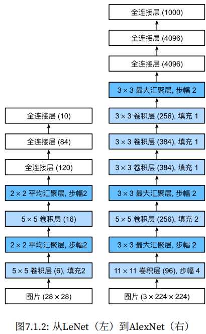
深度卷积神经网络AlexNet AlexNet相对LeNet的特点就是层数变得更深了,参数变得更多了。AlexNet由八层组成:五个卷积层、两个全连接隐藏层和一个全连接输出层。AlexNet使用ReLU而不是sigmoid作为其激活函数。 import torch from torch import nn from d2l import torch as d2l net = nn.Sequential( nn.Conv2d(1, 966, kernel_size=11, stride=4, padding=1), nn.ReLU(), nn.MaxPool2d(kernel_size=3, stride=2), nn.Conv2d(96, 256, kernel_size=5, padding=2), nn.ReLU(), nn.MaxPool2d(kernel_size=3, stride=2), nn.Conv2d(256, 384, kernel_size=3, padding=1), nn.ReLU(), nn.Conv2d(384, 384, kernel_size=3, padding=1), nn.ReLU(), nn.Conv2d(384, 256, kernel_size=3, padding=1), nn.ReLU(), nn.MaxPool2d(kernel_size=3, stride=2), nn.Flatten(), nn.Linear(6400, 4096), nn.ReLU(), nn ) X = torch.randn(1, 1, 224, 224) for layer in net: X=layer(X) print(layer.__class__.__name__,'output shape:\t',X.shape) 示例结果: Conv2d output shape: torch.Size([1, 96, 54, 54]) ReLU output shape: torch.Size([1, 96, 54, 54]) MaxPool2d output shape: torch.Size([1, 96, 26, 26]) Conv2d output shape: torch.Size([1, 256, 26, 26]) ReLU output shape: torch.Size([1, 256, 26, 26]) MaxPool2d output shape: torch.Size([1, 256, 12, 12]) Conv2d output shape: torch.Size([1, 384, 12, 12]) ReLU output shape: torch.Size([1, 384, 12, 12]) Conv2d output shape: torch.Size([1, 384, 12, 12]) ReLU output shape: torch.Size([1, 384, 12, 12]) Conv2d output shape: torch.Size([1, 256, 12, 12]) ReLU output shape: torch.Size([1, 256, 12, 12]) MaxPool2d output shape: torch.Size([1, 256, 5, 5]) Flatten output shape: torch.Size([1, 6400]) Linear output shape: torch.Size([1, 4096]) ReLU output shape: torch.Size([1, 4096]) Dropout output shape: torch.Size([1, 4096]) Linear output shape: torch.Size([1, 4096]) ReLU output shape: torch.Size([1, 4096]) Dropout output shape: torch.Size([1, 4096]) Linear output shape: torch.Size([1, 10]) AlexNet是更大更深的LeNet,比LeNet多了10倍的参数,260倍的计算复杂度。同时添加了丢弃法和ReLU。 使用块的网络VGG 通过AlexNet实践,添加更多的层使得模型的效果更好,但是要添加多少层了?是否有一些通用模版可以提供指导,VGG块就是解决这样的问题。将一些列的卷积层封装为一个块方便调用。 import torch from torch import nn from d2l import torch as d2l def vgg_block(num_convs, in_channels, out_channels): layers = [] for _ in range(num_convs): layers.append(nn.Conv2d(in_channels, out_channels, kernel_size=3, padding=1)) layers.append(nn.ReLU()) in_channels = out_channels layers.append(nn.MaxPool2d(kernel_size=2,stride=2)) return nn.Sequential(*layers) def vgg(conv_arch): conv_blks = [] in_channels = 1 # 卷积层部分 for (num_convs, out_channels) in conv_arch: conv_blks.append(vgg_block(num_convs, in_channels, out_channels)) in_channels = out_channels return nn.Sequential( *conv_blks, nn.Flatten(), # 全连接层部分 nn.Linear(out_channels * 7 * 7, 4096), nn.ReLU(), nn.Dropout(0.5), nn.Linear(4096, 4096), nn.ReLU(), nn.Dropout(0.5), nn.Linear(4096, 10)) conv_arch = ((1, 64), (1, 128), (2, 256), (2, 512), (2, 512)) net = vgg(conv_arch) X = torch.randn(size=(1, 1, 224, 224)) for blk in net: X = blk(X) print(blk.__class__.__name__,'output shape:\t',X.shape) 运行结果: Sequential output shape: torch.Size([1, 64, 112, 112]) Sequential output shape: torch.Size([1, 128, 56, 56]) Sequential output shape: torch.Size([1, 256, 28, 28]) Sequential output shape: torch.Size([1, 512, 14, 14]) Sequential output shape: torch.Size([1, 512, 7, 7]) Flatten output shape: torch.Size([1, 25088]) Linear output shape: torch.Size([1, 4096]) ReLU output shape: torch.Size([1, 4096]) Dropout output shape: torch.Size([1, 4096]) Linear output shape: torch.Size([1, 4096]) ReLU output shape: torch.Size([1, 4096]) Dropout output shape: torch.Size([1, 4096]) Linear output shape: torch.Size([1, 10]) VGG是使用可重复使用的卷积块来构建深度卷积神经网络,不同卷积块的个数和超参数可以得到不同复杂度的变种。 网络中的网络NiN 使用卷积层可以减少训练的参数。但从前面AlexNet或者VGG的示例中,卷积层后面全连接层参数是比较大的 LeNet: 1655*120 = 48K AlexNet: 25655*4096 = 26M VGG: 51277*4096 = 102M 哪有没有什么办法可以替换到全连接以减少参数?方法就是将全连接层替换为1*1的卷积层也可以起到全连接层的作用。 import torch from torch import nn from d2l import torch as d2l def nin_block(in_channels, out_channels, kernel_size, strides, padding): return nn.Sequential( nn.Conv2d(in_channels, out_channels, kernel_size, strides, padding), nn.ReLU(), nn.Conv2d(out_channels, out_channels, kernel_size=1), nn.ReLU(), nn.Conv2d(out_channels, out_channels, kernel_size=1), nn.ReLU()) net = nn.Sequential( nin_block(1, 96, kernel_size=11, strides=4, padding=0), nn.MaxPool2d(3, stride=2), nin_block(96, 256, kernel_size=5, strides=1, padding=2), nn.MaxPool2d(3, stride=2), nin_block(256, 384, kernel_size=3, strides=1, padding=1), nn.MaxPool2d(3, stride=2), nn.Dropout(0.5), # 标签类别数是10 nin_block(384, 10, kernel_size=3, strides=1, padding=1), nn.AdaptiveAvgPool2d((1, 1)), # 将四维的输出转成二维的输出,其形状为(批量大小,10) nn.Flatten()) X = torch.rand(size=(1, 1, 224, 224)) for layer in net: X = layer(X) print(layer.__class__.__name__,'output shape:\t', X.shape) 运行结果: Sequential output shape: torch.Size([1, 96, 54, 54]) MaxPool2d output shape: torch.Size([1, 96, 26, 26]) Sequential output shape: torch.Size([1, 256, 26, 26]) MaxPool2d output shape: torch.Size([1, 256, 12, 12]) Sequential output shape: torch.Size([1, 384, 12, 12]) MaxPool2d output shape: torch.Size([1, 384, 5, 5]) Dropout output shape: torch.Size([1, 384, 5, 5]) Sequential output shape: torch.Size([1, 10, 5, 5]) AdaptiveAvgPool2d output shape: torch.Size([1, 10, 1, 1]) Flatten output shape: torch.Size([1, 10]) NiN块使用卷积层加两个1*1卷积层,整个架构没有全连接层,降低了参数的数量。 并行连结的网络GoogleNet 在goodLeNet,基本的卷积块称为Inception块,有四条并行路径组成。googleNet类似于滤波器的组合,可以用各种滤波器尺寸探索图像,不同大小的滤波器可以有效识别不同范围的图像细节。 import torch from torch import nn from torch.nn import functional as F from d2l import torch as d2l class Inception(nn.Module): # c1--c4是每条路径的输出通道数 def __init__(self, in_channels, c1, c2, c3, c4, **kwargs): super(Inception, self).__init__(**kwargs) # 线路1,单1x1卷积层 self.p1_1 = nn.Conv2d(in_channels, c1, kernel_size=1) # 线路2,1x1卷积层后接3x3卷积层 self.p2_1 = nn.Conv2d(in_channels, c2[0], kernel_size=1) self.p2_2 = nn.Conv2d(c2[0], c2[1], kernel_size=3, padding=1) # 线路3,1x1卷积层后接5x5卷积层 self.p3_1 = nn.Conv2d(in_channels, c3[0], kernel_size=1) self.p3_2 = nn.Conv2d(c3[0], c3[1], kernel_size=5, padding=2) # 线路4,3x3最大汇聚层后接1x1卷积层 self.p4_1 = nn.MaxPool2d(kernel_size=3, stride=1, padding=1) self.p4_2 = nn.Conv2d(in_channels, c4, kernel_size=1) def forward(self, x): p1 = F.relu(self.p1_1(x)) p2 = F.relu(self.p2_2(F.relu(self.p2_1(x)))) p3 = F.relu(self.p3_2(F.relu(self.p3_1(x)))) p4 = F.relu(self.p4_2(self.p4_1(x))) # 在通道维度上连结输出 return torch.cat((p1, p2, p3, p4), dim=1) b1 = nn.Sequential(nn.Conv2d(1, 64, kernel_size=7, stride=2, padding=3), nn.ReLU(), nn.MaxPool2d(kernel_size=3, stride=2, padding=1)) b2 = nn.Sequential(nn.Conv2d(64, 64, kernel_size=1), nn.ReLU(), nn.Conv2d(64, 192, kernel_size=3, padding=1), nn.ReLU(), nn.MaxPool2d(kernel_size=3, stride=2, padding=1)) b3 = nn.Sequential(Inception(192, 64, (96, 128), (16, 32), 32), Inception(256, 128, (128, 192), (32, 96), 64), nn.MaxPool2d(kernel_size=3, stride=2, padding=1)) b4 = nn.Sequential(Inception(480, 192, (96, 208), (16, 48), 64), Inception(512, 160, (112, 224), (24, 64), 64), Inception(512, 128, (128, 256), (24, 64), 64), Inception(512, 112, (144, 288), (32, 64), 64), Inception(528, 256, (160, 320), (32, 128), 128), nn.MaxPool2d(kernel_size=3, stride=2, padding=1)) b5 = nn.Sequential(Inception(832, 256, (160, 320), (32, 128), 128), Inception(832, 384, (192, 384), (48, 128), 128), nn.AdaptiveAvgPool2d((1,1)), nn.Flatten()) net = nn.Sequential(b1, b2, b3, b4, b5, nn.Linear(1024, 10)) X = torch.rand(size=(1, 1, 96, 96)) for layer in net: X = layer(X) print(layer.__class__.__name__,'output shape:\t', X.shape) 运行结果: Sequential output shape: torch.Size([1, 64, 24, 24]) Sequential output shape: torch.Size([1, 192, 12, 12]) Sequential output shape: torch.Size([1, 480, 6, 6]) Sequential output shape: torch.Size([1, 832, 3, 3]) Sequential output shape: torch.Size([1, 1024]) Linear output shape: torch.Size([1, 10]) inception块用了4条有不同超参数的卷积层和池化层的路来抽取不同的信息,它主要的优点事模型参数小,计算复杂度第,googleNet用了9个Inception块,是第一个达到上百层的网络。 批量归一化 批量归一化(Batch Normalization,简称BN)是一种在训练神经网络时用于加速收敛、提高模型稳定性和提高性能的技术。它通过规范化每一层的输入,确保每一层的输入具有相同的分布,从而减少了不同层之间数据分布的变化,避免了梯度消失或爆炸问题。 具体来说,批量归一化的过程如下: 计算均值和方差:对于每一层的输入,计算该层在一个小批量(batch)上的均值和方差。通常是在训练过程中,对每个特征(特征是指每一维数据)独立地计算均值和方差。 归一化:利用上述计算出的均值和方差,对输入数据进行归一化。每个输入的值减去该批量的均值并除以该批量的标准差,从而将输入的分布调整为均值为0,方差为1的标准正态分布。 缩放与偏移:归一化后的数据会通过一个可学习的参数进行缩放(scale)和偏移(shift),即引入两个新的参数:γ(gamma)和β(beta)。这些参数允许模型恢复某些可能丢失的信息。 简单理解批量归一化就是对输入的数据按照按照小批量的均值、方差、$\boldsymbol{\gamma}$和$\boldsymbol{\beta}$的公式进行处理,得到输出后的数据。这样也相当于对输入的数据加入了噪音,因此不要和丢弃法混合使用。 $$\mathrm{BN}(\mathbf{x}) = \boldsymbol{\gamma} \odot \frac{\mathbf{x} - \hat{\boldsymbol{\mu}}\mathcal{B}}{\hat{\boldsymbol{\sigma}}\mathcal{B}} + \boldsymbol{\beta}.$$ $\hat{\boldsymbol{\mu}}_\mathcal{B}$:是小批量 $\mathcal{B}$的样本均值 $\hat{\boldsymbol{\sigma}}_\mathcal{B}$:是小批量$\mathcal{B}$的样本标准差。 由于单位方差(与其他一些魔法数)是一个主观的选择,因此我们通常包含拉伸参数(scale)$\boldsymbol{\gamma}$和偏移参数(shift)$\boldsymbol{\beta}$,它们的形状与$\mathbf{x}$相同。需要注意的是,$\boldsymbol{\gamma}$和$\boldsymbol{\beta}$是需要与其他模型参数一起学习的参数。 由于在训练过程中,中间层的变化幅度不能过于剧烈,而批量规范化将每一层主动居中,并将它们重新调整为给定的平均值和大小。 如下所示: net = nn.Sequential( nn.Conv2d(1, 6, kernel_size=5), BatchNorm(6, num_dims=4), nn.Sigmoid(), nn.AvgPool2d(kernel_size=2, stride=2), nn.Conv2d(6, 16, kernel_size=5), BatchNorm(16, num_dims=4), nn.Sigmoid(), nn.AvgPool2d(kernel_size=2, stride=2), nn.Flatten(), nn.Linear(16*4*4, 120), BatchNorm(120, num_dims=2), nn.Sigmoid(), nn.Linear(120, 84), BatchNorm(84, num_dims=2), nn.Sigmoid(), nn.Linear(84, 10)) 上面的示例中,在卷积层的后面使用了BatchNorm(6, num_dims=4)批量归一化。批量归一化就是固定小批量中的均值和方差,然后学习出适合的偏移和缩放,这样可以加速手链速度,但一般不改变模型的精度 残差网络ResNet 使用残差可以使得模型可以容易得叠加很多层,先来看看,什么是残差网络?残差网络就是由一系列的残差块组成,下图就是一个残差块。用公式表示就是:$X_{l+1} = X_l + F(X_l, W_l)$,,其中$F(X_l, W_l)$是残差。 残差块分有直接映射+残差两部分组成,表示输入经过残差块或直接映射到底输出。 在传统的神经网络中,输入$ X $会经过多层变换(如卷积、激活等),最终得出输出$ Y $。这些变换会逐渐改变输入的信息,试图将其转化为输出的目标形式。而在残差网络中,模型不仅学习输入$ X $到输出 $ Y $的映射,而是学习输入和输出之间的差异,即残差。数学上,可以表示为: $$ Y' = X + F(X) $$ 其中,$ Y' $是网络的最终输出,$ F(X) $ 是通过多个层(如卷积层、激活层等)处理后的结果(这个部分是“残差”),而 $ X $是输入。这里,$ F(X) $ 就是输入 $ X $与输出$ Y $之间的差异。也就是说X加上一个什么样的函数,能逼近Y。 为什么学习残差更容易? 学习从输入到输出的直接映射可能很复杂,特别是在深层网络中,因为输入经过多次变换后,最终的输出可能与输入有很大的差异。传统网络需要学习整个映射过程,这样可能导致训练时出现梯度消失或信息丢失的问题。但是,学习输入和输出之间的残差通常更简单。因为,通常情况下,输入和输出之间的差异(残差)可能是一个相对较小且较简单的函数。这使得网络能更容易捕捉到输入与输出之间的“偏差”,而不是直接学习整个变换过程。 举个例子 假设我们有一个非常深的网络,输入 $ X $ 和目标输出 $ Y $ 之间的关系很复杂。传统的网络可能需要直接学习一个非常复杂的映射函数。与此不同,残差网络并不直接学习这个复杂的映射,而是学习输入 $ X $ 和输出 $ Y $ 之间的差异。 例如,如果输出 $ Y $ 只是输入 $ X $ 加上一个小的偏差(例如,$ Y = X + \epsilon $),那么残差 $ F(X) = \epsilon $ 就是一个简单的学习目标。这个“差异”往往比直接学习整个映射来得容易。 可以把残差看作是一个补充信息。例如,假设你有一个图片分类任务,输入是图片,输出是类别标签。传统网络要直接将图片映射到标签,这个过程非常复杂。而在残差网络中,网络实际上在学习的是“这张图片与类别标签之间的差异”。如果输入与输出之间的关系可以通过一个小的差异来描述,那么网络只需要学习这个差异,训练起来会更容易。 残差网络的关键在于它将学习的重点从直接映射 $ X \to Y $ 转变为学习输入和输出之间的差异(残差) $ F(X) $。这样,网络不仅能更加高效地训练,还能避免深层网络中常见的梯度消失和信息衰减问题。 上图有两个残差块,左图中X可以直接到输出,右图中X经过1*1 Conv层到输出。对于左图当虚线框中的块如果是0,那么X还是原来的X。通过残差在在计算梯度时,可以使得接近输入层的参数可以得到更好的训练,因为经过多层神经网络后,最后一层可以通过“捷径”直到前面的层,这样梯度计算就更方便。 使用残差可以高效的训练靠近输入的神经网络的参数,避免层数的加深,越靠近输入的神经网络层参数变化较小而导致难以训练,因为梯度的计算是从后往前,而最后的参数如果相对较小时,通过链式法则计算(相乘)的前面梯度会更小,也就是前面层数w变化就小。 import torch from torch import nn from torch.nn import functional as F from d2l import torch as d2l class Residual(nn.Module): #@save def __init__(self, input_channels, num_channels, use_1x1conv=False, strides=1): super().__init__() self.conv1 = nn.Conv2d(input_channels, num_channels, kernel_size=3, padding=1, stride=strides) self.conv2 = nn.Conv2d(num_channels, num_channels, kernel_size=3, padding=1) if use_1x1conv: self.conv3 = nn.Conv2d(input_channels, num_channels, kernel_size=1, stride=strides) else: self.conv3 = None self.bn1 = nn.BatchNorm2d(num_channels) self.bn2 = nn.BatchNorm2d(num_channels) def forward(self, X): Y = F.relu(self.bn1(self.conv1(X))) Y = self.bn2(self.conv2(Y)) if self.conv3: X = self.conv3(X) Y += X #---------------->核心算法 return F.relu(Y) #构建一个残差块 def resnet_block(input_channels, num_channels, num_residuals, first_block=False): blk = [] for i in range(num_residuals): if i == 0 and not first_block: blk.append(Residual(input_channels, num_channels, use_1x1conv=True, strides=2)) else: blk.append(Residual(num_channels, num_channels)) return blk b1 = nn.Sequential(nn.Conv2d(1, 64, kernel_size=7, stride=2, padding=3), nn.BatchNorm2d(64), nn.ReLU(), nn.MaxPool2d(kernel_size=3, stride=2, padding=1)) #b2~b5是残差块生成 b2 = nn.Sequential(*resnet_block(64, 64, 2, first_block=True)) b3 = nn.Sequential(*resnet_block(64, 128, 2)) b4 = nn.Sequential(*resnet_block(128, 256, 2)) b5 = nn.Sequential(*resnet_block(256, 512, 2)) net = nn.Sequential(b1, b2, b3, b4, b5, nn.AdaptiveAvgPool2d((1,1)), nn.Flatten(), nn.Linear(512, 10)) X = torch.rand(size=(1, 1, 224, 224)) for layer in net: X = layer(X) print(layer.__class__.__name__,'output shape:\t', X.shape) 运行结果: Sequential output shape: torch.Size([1, 64, 56, 56]) Sequential output shape: torch.Size([1, 64, 56, 56]) Sequential output shape: torch.Size([1, 128, 28, 28]) Sequential output shape: torch.Size([1, 256, 14, 14]) Sequential output shape: torch.Size([1, 512, 7, 7]) AdaptiveAvgPool2d output shape: torch.Size([1, 512, 1, 1]) Flatten output shape: torch.Size([1, 512]) Linear output shape: torch.Size([1, 10]) Sequential( (0): Sequential( (0): Conv2d(1, 64, kernel_size=(7, 7), stride=(2, 2), padding=(3, 3)) (1): BatchNorm2d(64, eps=1e-05, momentum=0.1, affine=True, track_running_stats=True) (2): ReLU() (3): MaxPool2d(kernel_size=3, stride=2, padding=1, dilation=1, ceil_mode=False) ) (1): Sequential( (0): Residual( (conv1): Conv2d(64, 64, kernel_size=(3, 3), stride=(1, 1), padding=(1, 1)) (conv2): Conv2d(64, 64, kernel_size=(3, 3), stride=(1, 1), padding=(1, 1)) (bn1): BatchNorm2d(64, eps=1e-05, momentum=0.1, affine=True, track_running_stats=True) (bn2): BatchNorm2d(64, eps=1e-05, momentum=0.1, affine=True, track_running_stats=True) ) (1): Residual( (conv1): Conv2d(64, 64, kernel_size=(3, 3), stride=(1, 1), padding=(1, 1)) (conv2): Conv2d(64, 64, kernel_size=(3, 3), stride=(1, 1), padding=(1, 1)) (bn1): BatchNorm2d(64, eps=1e-05, momentum=0.1, affine=True, track_running_stats=True) (bn2): BatchNorm2d(64, eps=1e-05, momentum=0.1, affine=True, track_running_stats=True) ) ) (2): Sequential( (0): Residual( (conv1): Conv2d(64, 128, kernel_size=(3, 3), stride=(2, 2), padding=(1, 1)) (conv2): Conv2d(128, 128, kernel_size=(3, 3), stride=(1, 1), padding=(1, 1)) (conv3): Conv2d(64, 128, kernel_size=(1, 1), stride=(2, 2)) (bn1): BatchNorm2d(128, eps=1e-05, momentum=0.1, affine=True, track_running_stats=True) (bn2): BatchNorm2d(128, eps=1e-05, momentum=0.1, affine=True, track_running_stats=True) ) (1): Residual( (conv1): Conv2d(128, 128, kernel_size=(3, 3), stride=(1, 1), padding=(1, 1)) (conv2): Conv2d(128, 128, kernel_size=(3, 3), stride=(1, 1), padding=(1, 1)) (bn1): BatchNorm2d(128, eps=1e-05, momentum=0.1, affine=True, track_running_stats=True) (bn2): BatchNorm2d(128, eps=1e-05, momentum=0.1, affine=True, track_running_stats=True) ) ) (3): Sequential( (0): Residual( (conv1): Conv2d(128, 256, kernel_size=(3, 3), stride=(2, 2), padding=(1, 1)) (conv2): Conv2d(256, 256, kernel_size=(3, 3), stride=(1, 1), padding=(1, 1)) (conv3): Conv2d(128, 256, kernel_size=(1, 1), stride=(2, 2)) (bn1): BatchNorm2d(256, eps=1e-05, momentum=0.1, affine=True, track_running_stats=True) (bn2): BatchNorm2d(256, eps=1e-05, momentum=0.1, affine=True, track_running_stats=True) ) (1): Residual( (conv1): Conv2d(256, 256, kernel_size=(3, 3), stride=(1, 1), padding=(1, 1)) (conv2): Conv2d(256, 256, kernel_size=(3, 3), stride=(1, 1), padding=(1, 1)) (bn1): BatchNorm2d(256, eps=1e-05, momentum=0.1, affine=True, track_running_stats=True) (bn2): BatchNorm2d(256, eps=1e-05, momentum=0.1, affine=True, track_running_stats=True) ) ) (4): Sequential( (0): Residual( (conv1): Conv2d(256, 512, kernel_size=(3, 3), stride=(2, 2), padding=(1, 1)) (conv2): Conv2d(512, 512, kernel_size=(3, 3), stride=(1, 1), padding=(1, 1)) (conv3): Conv2d(256, 512, kernel_size=(1, 1), stride=(2, 2)) (bn1): BatchNorm2d(512, eps=1e-05, momentum=0.1, affine=True, track_running_stats=True) (bn2): BatchNorm2d(512, eps=1e-05, momentum=0.1, affine=True, track_running_stats=True) ) (1): Residual( (conv1): Conv2d(512, 512, kernel_size=(3, 3), stride=(1, 1), padding=(1, 1)) (conv2): Conv2d(512, 512, kernel_size=(3, 3), stride=(1, 1), padding=(1, 1)) (bn1): BatchNorm2d(512, eps=1e-05, momentum=0.1, affine=True, track_running_stats=True) (bn2): BatchNorm2d(512, eps=1e-05, momentum=0.1, affine=True, track_running_stats=True) ) ) (5): AdaptiveAvgPool2d(output_size=(1, 1)) (6): Flatten(start_dim=1, end_dim=-1) (7): Linear(in_features=512, out_features=10, bias=True) ) 本文来自: <动手学深度学习 V2> 的学习笔记 -

卷积神经网络CNN
图像卷积 图像卷积是有一个卷积核,这个卷积核对输入做相关运算。卷积核从输入的张量左上角开始、从左到右、从上到下进行滑动,每到一个位置时,在该窗口的部分张量与卷积核做点积得到一个输出。 为什么要使用卷积了,主要是要解决以下问题 参数爆炸问:传统全连接网络处理图像时参数规模过大(如1000×1000像素图像需30亿参数),而CNN通过局部连接和权值共享大幅减少参数数量23。 平移不变性缺:卷积核的滑动扫描机制使CNN能识别不同位置的相同特征。 局部相关性建:通过卷积操作捕捉相邻像素间的空间关联性。 如果是多个输入通道,比如图片RGB 3个通道,那么核函数对应有3个核函数,下面是2个通道的示例。 卷积核放在神经网络里,就代表对应的权重(weight),卷积网络可以起到提取图像特征的作用。 池化pooling 在处理图像时,每个像素的变化会导致参数变化也比较大,随着神经网络层数的上升,每个神经元对其敏感的感受就越大,这样对训练不一定是件好事情。为了减低卷积层对位置的敏感性,可以通过再加一层池化层来解决,池化一般有最大值和平均值两种方法。 maximum pooling: 取池化层窗口的最大值 average pooling: 取池化层窗口的平均值。 池化层与卷积的运算类似,只不过运算不一样。池化窗口从输入张量的左上角开始、从左往右、从上往下的在输入张量内滑动。在池化窗口达到的位置,计算该窗口的子张量最大值或者平均值。 LeNet网络 LeNet是最早的卷积神经网络,在1989年广泛运用在自动取款机中。 import torch from torch import nn from d2l import torch as d2l net = nn.Sequential( nn.Conv2d(1, 6, kernel_size=5, padding=2), nn.Sigmoid(), #第一个参数1表示输入通道,6表示输出通道。这里的通道指的 nn.AvgPool2d(kernel_size=2, stride=2), nn.Conv2d(6, 16, kernel_size=5), nn.Sigmoid(), nn.AvgPool2d(kernel_size=2, stride=2), nn.Flatten(), nn.Linear(16 * 5 * 5, 120), nn.Sigmoid(), nn.Linear(120, 84), nn.Sigmoid(), nn.Linear(84, 10)) 本文来自: <动手学深度学习 V2> 的学习笔记 -
层与块
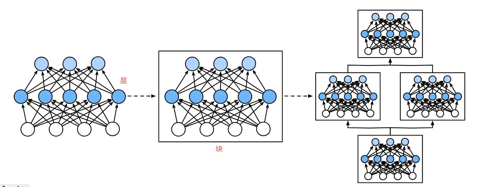
简单来说,如下图,第一个图中间5个神经元组成了一个层。第二图3个层组成了块。第三个图中3个块组成了整个模型。 层 层是神经网络的基本计算单元,负责对输入数据进行特定形式的变换,如线性映射、非线性激活等。其主要的功能是接收输入数据,生成输出结果。其中包含学习参数(如全连接层的权重和偏置)或无参数操作(如激活函数),输出形状可能与输入不同,例如全连接层将维度din映射到dout。 全连接层 layer = nn.Linear(4, 5) # 输入维度4,输出维度5 X = torch.randn(3, 4) # 输入形状(3,4) output = layer(X) # 输出形状(3,5) :ml-citation{ref="1,3" data="citationList"} nn.Linerar(4, 5):这里传入两个参数,第一个参数表示输入数据特征维度(示例是4),第二个参数表示输出特征维度(示例是5)。注意这里是特征维度,而不是样本个数,比如这里的特征维度是4,可以输入[2,4],[6,4]即2行4列或6行4列的数据样本。 激活函数层 layer = nn.ReLU() # 无参数操作 output = layer(torch.tensor([-1, 2, -3])) # 输出[0, 2, 0] :ml-citation{ref="3,5" data="citationList"} 激活函数层也是单独的一层。激活函数层是神经网络中用于引入非线性的部分,它的作用是帮助网络学习到更加复杂的函数映射。没有激活函数,神经网络只能表示线性函数,而引入非线性后,神经网络可以表示更复杂的模式,从而在各种任务(如分类、回归等)中表现得更好。 自定义层 在神经网络中,自定义层是用户根据具体任务需求自定义实现的层。与内置层(全连接层、卷积层)不同,自定义层可以根据特定的逻辑或行为来扩展模型。它允许你在训练和推理过程中执行特殊的操作或改变标准层的行为。使用自定义层可以使某些模型进行特殊计算,比如自定义正则化、损失函数或特殊的激活函数等。 在pytorch中如何实现自定义层,通常是通过继承torch.nn.Module类来实现的,需要定义的内容如下: init:定义层需要的参数或子层。 forward:定义数据如何通过该层传递并执行相应的计算。 无参数层 无参数层不包含任何需要训练的参数,通常用于执行某些固定的操作或计算。比如激活函数、归一化操作、数学变换等。 import torch import torch.nn as nn #继承nn.Module class custom_relu(nn.Module): def __init__(self): super().__init__() def forward(self, x): return torch.maximum(x, torch.tensor(0.0)) layer = custom_relu() input_data = torch.randn(3, 3) print(input_data) output_data = layer(input_data) print(output_data) 代码运行结果如下: tensor([[ 0.9986, -0.8549, -0.2031], [ 0.8380, 0.6925, -0.9164], [ 0.5807, -0.5719, 1.1864]]) tensor([[0.9986, 0.0000, 0.0000], [0.8380, 0.6925, 0.0000], [0.5807, 0.0000, 1.1864]]) 带参数的层 参数层包含可学习的按时,通常执行一些依赖于权重或偏置的计算,比如线性变换、卷积等。参数层通常会在训练过程中优化这些参数。 import torch import torch.nn as nn class custom_linear_layer(nn.Module): def __init__(self, input_dim, output_dim): super().__init__() self.weights = nn.Parameter(torch.randn(input_dim, output_dim)) self.bias = nn.Parameter(torch.randn(output_dim)) def forward(self, x): return torch.matmul(x, self.weights) + self.bias layer = custom_linear_layer(3, 2) input_data = torch.randn(5, 3) print(input_data) output_data = layer(input_data) print(output_data) 运行结果如下: tensor([[-0.7047, 1.8763, 1.8934], [-0.1341, 0.4411, 0.2252], [ 1.0531, 0.2556, -0.0045], [-0.9485, 1.9396, -0.3373], [-0.4364, 0.4522, -0.3176]]) tensor([[ 2.2790, -0.5707], [ 0.0157, -0.3939], [-0.7449, -0.6362], [ 0.1973, -1.3335], [-0.3929, -0.5201]], grad_fn=<AddBackward0>) 块 块是由多个层组成的复合模块,用于封装重复或复杂功能的代码逻辑,实现模型结构的模块化。包含前向传播逻辑forward的方法、可嵌套其他块或层形成层次化的结构,继承自nn.Module,支持参数管理和自动梯度计算。 Sequential容器 block = nn.Sequential( nn.Linear(4, 5), nn.ReLU(), nn.Linear(5, 3) ) # 包含3个子层:线性→激活→线性 :ml-citation{ref="6,7" data="citationList"} Sequential容器用于按顺序定义一个神经网络模块,它将各个子模块按照定义顺序组合在一起,从而实现前向传播。 输入:假设输入时一个形状为(batch_size, 4)的张量,表示batch_size个样本,每个样本有4个特征。 第一个线性层:输入通过第一个nn.Linear(4, 5), 输出形状变为(batch_size, 5)。 ReLu激活函数:输出经过第一个nn.ReLU,所有负数变为0,正数保持不变,输出仍为形状(batch_size, 5)。 第二个线性层:经过第二个nn.Linear(5, 3),输出形状变为(batch_size, 3)。 import torch import torch.nn as nn block = nn.Sequential( nn.Linear(4, 5), # 输入样本是4个特征, 转换为5个特征 nn.ReLU(), nn.Linear(5, 3)) #输出3个特征 input_data = torch.randn(2, 4) print(input_data) output_data = block(input_data) print(output_data) 运行结果: tensor([[ 0.3054, 1.0160, -1.7137, -0.3744], [-0.6882, -0.3049, -1.2769, 0.2835]]) tensor([[ 0.4485, 0.6298, -0.1949], [ 0.1992, 0.1609, -0.2480]], grad_fn=<AddmmBackward0>) 自定义块 在pytorch中,自定义块通常是通过继承nn.Module创建的自定义或模型块。可以根据需要组合多个操作或实现一些特定功能,创建属于自己的网络模块。 如何创建自定义块了? 基层nn.Module: 需要先继承nn.Module,这是pytorch中所有神经网络模块的基类。 定义init方法:在init方法中定义层,例如nn.Linear、nn.Conv2d等操作并初始化他们。 定义forward方法:在forward方法中定义输入数据如何通过自定义层进行处理。 import torch import torch.nn as nn class custom_block(nn.Module): def __init__(self): super().__init__() self.fc1 = nn.Linear(4, 5) self.fc2 = nn.Linear(5, 3) self.relu = nn.ReLU() def forward(self, x): x = self.fc1(x) x = self.relu(x) x = self.fc2(x) return x custom_block = custom_block() input_data = torch.randn(2, 4) print(input_data) output_data = custom_block(input_data) print(output_data) 运行结果如下: tensor([[-0.4663, 0.9429, -0.2072, -1.7672], [ 0.6028, -0.2563, -0.3493, 1.2657]]) tensor([[-0.0273, -0.1265, -0.2595], [ 0.1276, -0.0837, -0.4265]], grad_fn=<AddmmBackward0>) 复杂块 待补充 参数管理 在深度学习中,参数管理通常指的是如何管理模块中的参数,确保它们在训练过程中得到适当的更新,或者在不同阶段(如训练、验证、测试)进行适当的操作。有效的参数管理有助于提高模型训练的效率和稳定性。 参数访问 import torch from torch import nn net = nn.Sequential( nn.Linear(4, 8), nn.ReLU(), nn.Linear(8, 1)) X = torch.rand(size=(2, 4)) y = net(X) print(y) print(net[2].state_dict()) print(type(net[2].bias)) print(net[2].bias) print(net[2].bias.data) print(net[2].weight.grad) 运行结果如下: tensor([[-0.1428], [-0.1919]], grad_fn=<AddmmBackward0>) OrderedDict([('weight', tensor([[-0.3178, -0.2009, -0.1120, 0.1502, 0.0054, -0.0864, 0.2142, -0.0564]])), ('bias', tensor([-0.0326]))]) #打印.state_dirct() <class 'torch.nn.parameter.Parameter'> #-打印.bias Parameter containing: tensor([-0.0326], requires_grad=True) tensor([-0.0326]) #打印.bias.data None #打印.weight.grad 也可以使用下面的一次性访问所有参数 print(*[(name, param.shape) for name, param in net[0].named_parameters()]) print(*[(name, param.shape) for name, param in net.named_parameters()]) 运行结果: ('weight', torch.Size([8, 4])) ('bias', torch.Size([8])) ('0.weight', torch.Size([8, 4])) ('0.bias', torch.Size([8])) ('2.weight', torch.Size([1, 8])) ('2.bias', torch.Size([1])) 另外可以使用print打印模型的结构 print(net) 运行如下: Sequential( (0): Linear(in_features=4, out_features=8, bias=True) (1): ReLU() (2): Linear(in_features=8, out_features=1, bias=True) ) 参数初始化 def init_normal(m): if type(m) == nn.Linear: nn.init.normal_(m.weight, mean=1, std=0.01) nn.init.zeros_(m.bias) net.apply(init_normal) net[0].weight.data[0], net[0].bias.data[0] 运行结果如下: (tensor([0.9942, 0.9995, 0.9971, 0.9903]), tensor(0.)) 上面的代码定义了一个init_normal函数,改变了weight和bias,初始化为标准差0.01的高斯随机变量且将参数设置为0。 参数绑定 所谓参数绑定,就是将多个层间使用共享参数,下面看示例。 shared = nn.Linear(8, 8) net = nn.Sequential(nn.Linear(4, 8), nn.ReLU(), shared, nn.ReLU(), shared, nn.ReLU(), nn.Linear(8, 1)) net(X) print(net) print(net[2].weight.data[0] == net[4].weight.data[0]) net[2].weight.data[0, 0] = 100 print(net[2].weight.data[0] == net[4].weight.data[0]) 运行结果如下: Sequential( (0): Linear(in_features=4, out_features=8, bias=True) (1): ReLU() (2): Linear(in_features=8, out_features=8, bias=True) (3): ReLU() (4): Linear(in_features=8, out_features=8, bias=True) (5): ReLU() (6): Linear(in_features=8, out_features=1, bias=True) ) tensor([True, True, True, True, True, True, True, True]) tensor([True, True, True, True, True, True, True, True]) 可以看到第2层和第4层的参数是一样的,他们不仅值相等,当改变其中一个参数,另一个参数也会一起改变为一样的值。 参数存储 在pytorch中可以调用save和load保存和读取文件,示例如下。 import torch from torch import nn from torch.nn import functional as F x = torch.arange(4) print(x) torch.save(x, 'x-file') x2 = torch.load('x-file') print(x2) 打印如下: tensor([0, 1, 2, 3]) tensor([0, 1, 2, 3]) 在训练过程中,可以将参数进行保存,下面是示例。 class nlp(nn.Module): def __init__(self): super().__init__() self.hidden = nn.Linear(20, 256) self.output = nn.Linear(256, 10) def forward(self, x): return self.output(F.relu(self.hidden(x))) net = nlp() print(net) X = torch.randn(size=(2, 20)) print(X) Y = net(X) print(Y) torch.save(net.state_dict(), 'nlp.params') clone = nlp() clone.load_state_dict(torch.load('nlp.params')) clone.eval Y_clone = clone(X) Y_clone == Y 打印结果: nlp( (hidden): Linear(in_features=20, out_features=256, bias=True) (output): Linear(in_features=256, out_features=10, bias=True) ) tensor([[-1.3927, -1.9475, -0.6044, -0.5835, -0.5661, -0.4240, -1.4481, -0.0627, 0.7437, 1.0465, 0.1806, 0.1096, -1.2199, 1.1642, 1.0633, 1.3925, 0.3849, 0.9443, -0.4781, 0.6522], [ 1.2506, -0.7369, 0.7148, -0.3734, 1.3801, 0.4163, -1.3707, 0.5407, -0.1734, -1.1068, -0.1630, 1.2899, 0.4753, 0.7332, 0.5401, -0.4011, -0.5356, -0.5833, 0.8288, -0.5439]]) tensor([[-0.6972, -0.0666, 0.5621, -0.4620, -0.1545, 0.2283, 0.1647, 0.1879, 0.1907, -0.1658], [-0.2174, 0.2586, 0.2867, -0.2213, -0.0090, 0.0687, -0.0382, -0.0477, -0.3194, 0.1438]], grad_fn=<AddmmBackward0>) tensor([[True, True, True, True, True, True, True, True, True, True], [True, True, True, True, True, True, True, True, True, True]]) 上面的示例中,先调用torch.save(net.state_dirc(), 'npl.params')将参数保存起来,然后接着通过load_state_dict(torch.load('npl.params')),将参数读取出来。通过保存参数的方法,可以将训练的实例化进行备份,从上一次保存的参数接着训练。 本文来自: <动手学深度学习 V2> 的学习笔记 -

Windows Ai开发环境安装
annaconda可以理解为ai环境可以创建很多个房间,比如允许多个不同版本的python。每个房间可以保存不同的环境变量。 步骤1:下载安装包,安装anaconda,https://www.anaconda.com/ 步骤2:设置环境变量 设置环境变量需要根据软件实际的安装位置,这里的软件是安装的D盘的。在cmd命令中,执行conda info表示设置环境变量成功。 步骤3: 创建环境 打开Anaconda Prompt终端界面,创建开发环境前,先更新清华的源。 conda config --add channels https://mirrors.tuna.tsinghua.edu.cn/anaconda/pkgs/free/ conda config --add channels https://mirrors.tuna.tsinghua.edu.cn/anaconda/pkgs/main/ conda config --add channels https://mirrors.tuna.tsinghua.edu.cn/anaconda/cloud/pytorch/ conda config --add channels https://mirrors.tuna.tsinghua.edu.cn/anaconda/cloud/pytorch/linux-64/ conda config --set show_channel_urls yes 然后进行安装: conda create -n py39_test python=3.9 -y 其中-n指定环境的名称, python=3.9表示安装python3.9的版本,-y表示同意所有安装过程中的所有确认。 步骤4: 激活环境 conda activate py39_test 步骤4:安装基础环境 pip install -r requirements.txt 使用pip install 进行安装,requirements.txt内容如下。 contourpy==1.3.0 cycler==0.12.1 filelock==3.16.1 fonttools==4.55.3 fsspec==2024.12.0 importlib_resources==6.5.2 Jinja2==3.1.5 kiwisolver==1.4.7 MarkupSafe==3.0.2 matplotlib==3.9.4 mpmath==1.3.0 networkx==3.2.1 numpy==2.0.2 packaging==24.2 pandas==2.2.3 pillow==11.1.0 pyparsing==3.2.1 python-dateutil==2.9.0.post0 pytz==2024.2 six==1.17.0 sympy==1.13.1 torch==2.5.1 torchaudio==2.5.1 torchvision==0.20.1 typing_extensions==4.12.2 tzdata==2024.2 zipp==3.21.0 使用pip list可以查看安装的包。 步骤5:安装pycharm,下载链接 https://www.jetbrains.com/pycharm/download/?section=windows -
前向传播、反向传播和计算图
前向传播(Forward Propagation) 前向传播是神经网络中从输入数据到输出预测值的计算过程。它通过逐层应用权重(W)和偏置(b),最终生成预测值 $y' $,并计算损失函数$L $。 模型定义 $$ y' = W \cdot x + b $$ 损失函数(均方误差) $$ L = \frac{1}{n} \sum_{i=1}^{n} (y'(i) - y_{\text{true}}(i))^2 $$ 示例 输入数据:$x = [1.0, 2.0] $ 真实标签:$y_{\text{true}} = [3.0, 5.0]$ 参数初始值:$W = 1.0, \, b = 0.5$ 前向计算 预测值:$y'(1) = 1.0 \cdot 1.0 + 0.5 = 1.5, \quad y'(2) = 1.0 \cdot 2.0 + 0.5 = 2.5$ 损失函数:$L = \frac{1}{2} \left[ (1.5 - 3)^2 + (2.5 - 5)^2 \right] = \frac{1}{2} (2.25 + 6.25) = 4.25$ 计算图(Computational Graph) 计算图是一种数据结构,用于表示前向传播中的计算过程。图中的节点代表数学操作(如加法、乘法),边代表数据流动(张量)。 对上述线性回归模型,计算图如下: 输入 x → (Multiply W) → (Add b) → 预测值 t_p → (Subtract y_true) → 误差平方 → 求和平均 → 损失 L 节点:乘法、加法、平方、求和、平均等操作。 边:数据流(如 $ x, W, b, y', L$)。 反向传播(Backward Propagation) 反向传播是通过链式法则(Chain Rule),从损失函数$ L $开始,反向计算每个参数$(W, b)$的梯度 $( \frac{\partial L}{\partial W} ) $和$ ( \frac{\partial L}{\partial b} ) $的过程。下面以线性回归模型公式示例: 损失对预测值的梯度 $$ \frac{\partial L}{\partial y'(i)} = \frac{2}{n} (y'(i) - y_{\text{true}}(i)) $$ 预测值对参数的梯度 对权重 $W $:$ \frac{\partial y'(i)}{\partial W} = x(i) $ 对偏置 $b $:$\frac{\partial y'(i)}{\partial b} = 1 $ 合并梯度 权重梯度:$ \frac{\partial L}{\partial W} = \sum_{i=1}^{n} \frac{\partial L}{\partial y'(i)} \cdot \frac{\partial y'(i)}{\partial W} = \frac{2}{n} \sum_{i=1}^{n} (y'(i) - y_{\text{true}}(i)) \cdot x(i) $ 偏置梯度:$ \frac{\partial L}{\partial b} = \sum_{i=1}^{n} \frac{\partial L}{\partial y'(i)} \cdot \frac{\partial y'(i)}{\partial b} = \frac{2}{n} \sum_{i=1}^{n} (y'(i) - y_{\text{true}}(i)) $ 反向传播示例 使用前向传播的结果: 计算误差项 $$ y'(1) - y_{\text{true}}(1) = 1.5 - 3 = -1.5, \quad y'(2) - y_{\text{true}}(2) = 2.5 - 5 = -2.5 $$ 计算梯度 权重梯度:$\frac{\partial L}{\partial W} = \frac{2}{2} [(-1.5) \cdot 1.0 + (-2.5) \cdot 2.0] = 1.0 \cdot (-1.5 - 5) = -6.5 $ 偏置梯度:$\frac{\partial L}{\partial b} = \frac{2}{2} [(-1.5) + (-2.5)] = 1.0 \cdot (-4) = -4$ PyTorch示例 import torch # 定义参数(启用梯度追踪) W = torch.tensor(1.0, requires_grad=True) b = torch.tensor(0.5, requires_grad=True) # 输入数据 x = torch.tensor([1.0, 2.0]) y_true = torch.tensor([3.0, 5.0]) # 前向传播 y_pred = W * x + b loss = torch.mean((y_pred - y_true) ** 2) # 反向传播 loss.backward() # 输出梯度 print(f"dL/dW: {W.grad}") # 输出 tensor(-6.5) print(f"dL/db: {b.grad}") # 输出 tensor(-4.0) 关键点说明 动态计算图:PyTorch 在前向传播时自动构建计算图。 反向传播触发:调用 .backward() 后,从损失节点反向遍历图,计算所有 requires_grad=True 的张量的梯度。 梯度存储:梯度结果存储在张量的 .grad 属性中。 总结: 概念 作用 示例中的体现 前向传播 计算预测值和损失函数 $ y' = W \cdot x + b, L = 4.25 $ 计算图 记录所有计算操作,为反向传播提供路径 乘法、加法、平方、求和、平均等操作组成的数据结构 反向传播 通过链式法则计算参数梯度 $ \frac{\partial L}{\partial W} = -6.5 $ 输入 x │ ▼ [W*x] → 乘法操作(计算图节点) │ ▼ [+b] → 加法操作(计算图节点) │ ▼ 预测值 y' → [平方损失] → 平均损失 L │ ▲ └──────────────────────────┘ 反向传播(梯度回传) -
梯度计算
什么是梯度 梯度(Gradient)是用于描述多元函数在某一点的变化率最大的方向及其大小。在深度学习中,梯度被广泛用于优化模型参数(如神经网络的权重和偏置),通过梯度下降等算法最小化损失函数。 对于多元函数 $f(x_1, x_2, \dots, x_n)$,其梯度是一个向量,由函数对每个变量的偏导数组成,记作: $$ \nabla f = \left( \frac{\partial f}{\partial x_1}, \frac{\partial f}{\partial x_2}, \dots, \frac{\partial f}{\partial x_n} \right) $$ 其中: $\nabla f$ 是梯度符号(读作“nabla f”)。 $\frac{\partial f}{\partial x_i}$ 是函数 $f$ 对变量 $x_i$ 的偏导数。 直观理解梯度 假设有一个二元函数 $f(x, y) = x^2 + y^2$,其梯度为: $$ \nabla f = \left( \frac{\partial f}{\partial x}, \frac{\partial f}{\partial y} \right) = (2x, 2y) $$ 在点 $(1, 1)$ 处,梯度为 $(2, 2)$,表示函数在该点沿方向 $(2, 2)$ 增长最快。 若想最小化 $f(x, y)$,应沿着负梯度方向 $-(2, 2)$ 移动,即更新参数: $$ x \leftarrow x - \alpha \cdot 2x $$ $$ y \leftarrow y - \alpha \cdot 2y $$ 其中 $\alpha$ 是学习率。 梯度在机器学习中的作用 在机器学习中,梯度表示损失函数(Loss Function)对模型参数的敏感度。例如,对于模型参数 $W$(权重)和 $b$(偏置),梯度 $\nabla L$ 包含两个分量: $$ \nabla L = \left( \frac{\partial L}{\partial W}, \frac{\partial L}{\partial b} \right) $$ 通过沿着负梯度方向更新参数(即梯度下降),可以逐步降低损失函数的值。 梯度下降的示例 目标:最小化函数 (线性回归的损失函数)。 $$ L(W, b) = (W \cdot x + b - y_{\text{true}})^2 $$ 假设 $$ x = 2, \quad y_{\text{true}} = 4, \quad W = 1, \quad b = 0.5 $$ 计算预测值: $$ y_{\text{pred}} = W \cdot x + b = 1 \cdot 2 + 0.5 = 2.5 $$ 计算损失: $$ L = (y_{\text{pred}} - y_{\text{true}})^2 = (2.5 - 4)^2 = 2.25 $$ 计算梯度: $$ \frac{\partial L}{\partial W} = 2 (y_{\text{pred}} - y_{\text{true}}) \cdot x = 2 (2.5 - 4) \cdot 2 = -6.0 $$ $$ \frac{\partial L}{\partial b} = 2 (y_{\text{pred}} - y_{\text{true}}) = 2 (2.5 - 4) = -3.0 $$ 梯度为 $$ \nabla L = (-6.0, -3.0) $$ 参数更新(学习率 $ (\alpha = 0.1))$: $$ W_{\text{new}} = W - \alpha \cdot \frac{\partial L}{\partial W} = 1 - 0.1 \cdot (-6.0) = 1.6 $$ $$ b_{\text{new}} = b - \alpha \cdot \frac{\partial L}{\partial b} = 0.5 - 0.1 \cdot (-3.0) = 0.8 $$ 梯度计算推导 这个公式是梯度计算中的一部分,计算的是损失函数 (L) 对参数 (W) 的偏导数。我们来一步步推导这个公式。 假设损失函数为: $$ L(W, b) = (W \cdot x + b - y_{\text{true}})^2 $$ 其中$ W$是权重,$b $是偏置,$x $是输入,$y_{\text{true}} $是真实的标签。我们要计算的是损失函数 $L$ 对权重 $W$的偏导数$ \frac{\partial L}{\partial W}$。 步骤 1: 定义损失函数 损失函数是预测值和真实值之间的误差的平方,定义为: $$ L(W, b) = (y_{\text{pred}} - y_{\text{true}})^2 $$ 其中,$y_{\text{pred}} = W \cdot x + b $是模型的预测值。这个损失函数是一个二次函数,目标是最小化它。 步骤 2: 使用链式法则求梯度 我们需要对损失函数 (L) 关于 (W) 求偏导数。首先可以应用链式法则: $$ \frac{\partial L}{\partial W} = \frac{\partial L}{\partial y_{\text{pred}}} \cdot \frac{\partial y_{\text{pred}}}{\partial W} $$ 步骤 3: 计算每一部分的偏导数 第一部分: 计算 $\frac{\partial L}{\partial y_{\text{pred}}}$。 由于损失函数是平方误差形式: $$ L = (y_{\text{pred}} - y_{\text{true}})^2 $$ 对$y_{\text{pred}}$求导,得到: $$ \frac{\partial L}{\partial y_{\text{pred}}} = 2(y_{\text{pred}} - y_{\text{true}}) $$ 第二部分: 计算 $\frac{\partial y_{\text{pred}}}{\partial W}$。 由于 $y_{\text{pred}} $= $W \cdot x + b$,对$ W $求导,得到: $$ \frac{\partial y_{\text{pred}}}{\partial W} = x $$ 步骤 4: 合并结果 现在将两部分结果结合起来: $$ \frac{\partial L}{\partial W} = 2(y_{\text{pred}} - y_{\text{true}}) \cdot x $$ 步骤 5: 将具体数值代入 根据给定的数值 $x = 2$,$ y_{\text{true}} = 4$, $W = 1$, 和 $b = 0.5$,我们首先计算预测值$y_{\text{pred}}$: $$ y_{\text{pred}} = W \cdot x + b = 1 \cdot 2 + 0.5 = 2.5 $$ 然后代入到梯度公式中: $$ \frac{\partial L}{\partial W} = 2(2.5 - 4) \cdot 2 = 2(-1.5) \cdot 2 = -6.0 $$ 所以,损失函数$ L$ 对 $W $的偏导数是 $-6.0$。 总结:对于复杂的梯度计算可以利用链式法则。在该示例中,先令 $y_{\text{pred}} $= $W \cdot x + b$。对$W$求偏导,就可以转化为,$\frac{\partial L}{\partial W} = \frac{\partial L}{\partial y_{\text{pred}}} \cdot \frac{\partial y_{\text{pred}}}{\partial W}$,然后可以先求$\frac{\partial L}{\partial y_{\text{pred}}} $,再求$\frac{\partial y_{\text{pred}}}{\partial W}$,这样计算就没有这么复杂了。根据公式$\frac{\partial L}{\partial y_{\text{pred}}} = 2(y_{\text{pred}} - y_{\text{true}})$,而$\frac{\partial y_{\text{pred}}}{\partial W} = x$,所以$\frac{\partial L}{\partial W} = 2(y_{\text{pred}} - y_{\text{true}}) \cdot x$,因此知道预测值、真实值、输入值、当前的权重和偏置即可算出偏导。同理$b$也可以用类似方法,继而算出损失函数的梯度$\nabla L = \left( \frac{\partial L}{\partial W}, \frac{\partial L}{\partial b} \right)$ pytorch示例 在pytorch中通过自动微分Autograd自动计算梯度,示例如下: import torch # 定义参数(启用梯度追踪) W = torch.tensor(1.0, requires_grad=True) b = torch.tensor(0.5, requires_grad=True) # 输入数据 x = torch.tensor(2.0) y_true = torch.tensor(4.0) # 前向传播 y_pred = W * x + b loss = (y_pred - y_true) ** 2 # 反向传播计算梯度 loss.backward() # 输出梯度 print(f"dL/dW: {W.grad}") # 输出 tensor(-6.0) print(f"dL/db: {b.grad}") # 输出 tensor(-3.0) 概念 数学表达 意义 梯度定义 ∇f = (∂f/∂x₁, …) 多元函数变化最快的方向及其速率 梯度下降 W ← W − α ⋅ ∂L/∂W 沿负梯度方向更新参数以最小化损失函数 PyTorch自动微分 loss.backward() 通过反向传播自动计算所有参数的梯度并存储在 .grad 中 -

激活函数
概念 前面我们主要使用的是线性模型,但是线性模型有很多局限性,因为我们要建模的问题并不能单纯使用线性模型就能够拟合的,如下示例。 我们要拟合红色部分的函数,使用线性模型即使在怎么调整W和b都没法进行拟合出来,要拟合这样的函数,我们需要非线性的函数。 如上图,要拟合这样的模型,我们可以使用①②③函数相加再加上一个b偏置。那这里的①②③函数怎么来了,可以看出是wx+b再经过一个sigmoid转换得来,那这里的sigmoid我们就称为激活函数。 激活函数的主要作用是引入非线性,使得神经网络能够处理更复杂的问题并避免退化成线性模型。没有激活函数,神经网络就无法发挥其强大的学习和表达能力。选择合适的激活函数对模型的训练和性能表现至关重要。 常见的激活函数 ReLU 激活函数 公式:$ \text{ReLU}(x) = \max(0, x) $ x = torch.arange(-8.0, 8.0, 0.1, requires_grad=True) y = torch.relu(x) d2l.plot(x.detach(), y.detach(), 'x', 'relu(x)', figsize=(5, 2.5)) ReLU激活函数用得比较多,因为其计算相对简单,不需要复杂的指数计算,因为指数计算都很贵。 ReLU函数进行求导,可以发现当输入为负时,导数为0,当输入为正是,导数为1。可以使用y.backward来计算导数,可以理解导数就是梯度。x取不同位置进行求导得到的值,就是相应位置的梯度。 y.backward(torch.ones_like(x), retain_graph=True) d2l.plot(x.detach(), x.grad, 'x', 'grad of relu', figsize=(5, 2.5)) Sigmoid 激活函数 公式: $ \sigma(x) = \frac{1}{1 + e^{-x}} $ y = torch.sigmoid(x) d2l.plot(x.detach(), y.detach(), 'x', 'sigmoid(x)', figsize=(5, 2.5)) Tanh 激活函数 公式: $ \tanh(x) = \frac{e^{x} - e^{-x}}{e^{x} + e^{-x}} $ y = torch.tanh(x) d2l.plot(x.detach(), y.detach(), 'x', 'tanh(x)', figsize=(5, 2.5)) Softmax 激活函数 公式: $ \text{Softmax}(z_i) = \frac{e^{z_i}}{\sum_{j=1}^{K} e^{z_j}} $ 在前面章节中,我们使用softmax用于线性回归的多分类,但其实softmax也可以看做一种激活函数。 softmax将神经网络的输出转换为概率分布,确保每个类别的输出值在0到1之间,且所有类别的概率和为1。如z=[2.0,1.0,0.1] 经过softmax计算转化后得[0.7,0.2,0.1],如果神经网络的输出为三个类别的得分,表示第一个类别的预测概率最大,约为70%。 总结来说,Softmax 是一种激活函数,它专门用于多分类问题的输出层,帮助模型生成一个概率分布,便于做分类决策。 -

sotfmax回归实现
什么是sotfmax回归 Softmax回归(Softmax Regression),也叫多项逻辑回归,是一种用于多分类问题的分类算法。它是对逻辑回归(Logistic Regression)的一种扩展,适用于处理输出类别数大于2的情况。Softmax回归通过使用Softmax函数来将每个类别的输出转化为一个概率分布,使得输出值能够表示每个类别的概率,并且所有类别的概率之和为1。 举个例子:假设有一个包含3个类别的多分类问题:苹果、香蕉、橙子。对于每个输入样本(例如一张图片),Softmax回归模型会输出三个值(每个类别的概率),也就是概率分布。例如: 苹果的概率:0.6 香蕉的概率:0.3 橙子的概率:0.1 这些概率加起来等于1,模型会将输入样本分类为苹果(因为概率最大)。 softmax函数 对于每个类别$ k $ ,我们会计算一个得分$ z_k $,然后将这个得分转化为概率。得分通常是由输入数据$ \mathbf{x} $与对应类别的权重向量$ \mathbf{w}_k $ 的线性组合给出的:$ z_k = \mathbf{w}_k^T \mathbf{x} + b_k $, 其中,$ \mathbf{w}_k $ 是第$ k$ 个类别的权重,$ b_k$ 是偏置项,$ \mathbf{x} $ 是输入特征向量。Softmax函数用于将这些得分$ z_k $转换成概率。 Softmax函数的形式如下:$ P(y = k | \mathbf{x}) = \frac{e^{z_k}}{\sum_{j=1}^K e^{z_j}} $ 。 $ P(y = k | \mathbf{x}) ) 是输入 ( \mathbf{x} $ 属于类别k的概率。 $ z_k $ 是类别 $ k $ 的得分。 $ \sum_{j=1}^K e^{z_j} $ 是所有类别得分的指数函数的和,确保概率和为1。 交叉熵损失函数 为了训练Softmax回归模型,我们使用交叉熵损失函数来评估模型预测与真实标签之间的差异。交叉熵损失函数的公式如下:$ L(\theta) = - \sum_{i=1}^N \sum_{k=1}^K y_{ik} \log P(y_k = 1 | \mathbf{x}_i) $ 其中: - $ N $ 是训练集中的样本数。 - $ y_{ik} $ 是样本 $ i $是否属于类别 $ k $ 的标签(通常是1或0)。 - $ P(y_k = 1 | \mathbf{x}_i) $ 是输入 $ \mathbf{x}_i $ 属于类别 $ k $ 的概率。 softmax实现示例 数据读取 pip install d2l==0.16 import torch from IPython import display from d2l import torch as d2l batch_size = 256 train_iter, test_iter = d2l.load_data_fashion_mnist(batch_size) 这里直接使用了d2l.load_data_fashion_mnist() 函数加载 Fashion-MNIST 数据集。load_data_fashion_mnist 是 d2l 库中的一个工具函数,用于加载 Fashion-MNIST 数据集并返回训练集和测试集的数据迭代器。train_iter 是训练集的迭代器。test_iter 是测试集的迭代器。数据迭代器是用于在模型训练和评估过程中批量加载数据的对象。batch_size 参数指定了每个批次包含多少个样本。 可以用下面的示例代码打印输入的数据 n = 10 for X, y in train_iter: break X_selected = X[0:n].reshape((n, 28, 28)) titles = [f'Label: {int(label)}' for label in y[0:n]] d2l.show_images(X_selected, 1, n, titles=titles) 定义模型 sotfmax函数 计算softmax的步骤如下: 对每个项求幂(使用exp) 对每一行求和(小批量中每个样本是一行),得到每个样本的规范化常数 将每一行除以其规范化常数,确保结果的和为1 def softmax(X): X_exp = torch.exp(X) print(X_exp) partition = X_exp.sum(1, keepdim=True) print(partition) return X_exp / partition 示例如下: X = torch.normal(0, 1, (2, 5)) #使用正态分布生成2行5列的矩阵 print(X) X_prob = softmax(X) X_prob, X_prob.sum(1) #生成的数据 tensor([[ 0.3141, 0.5186, -0.6949, 0.5918, -2.2370], [-0.3814, 0.8092, -0.1959, 0.7489, 1.8790]]) #torch.exp(X):对矩阵中每个数据求e^x指数运算后的结果 tensor([[1.3690, 1.6797, 0.4991, 1.8072, 0.1068], [0.6829, 2.2460, 0.8221, 2.1146, 6.5472]]) #X_exp.sum(1, keepdim=True): 对每一行求和 tensor([[ 5.4618], [12.4129]]) #将每一行除以其规范化常数,确保结果的和为1 (tensor([[0.2506, 0.3075, 0.0914, 0.3309, 0.0196], [0.0550, 0.1809, 0.0662, 0.1704, 0.5275]]), tensor([1., 1.])) 模型和参数 num_inputs = 784 num_outputs = 10 W = torch.normal(0, 0.01, size=(num_inputs, num_outputs), requires_grad=True) b = torch.zeros(num_outputs, requires_grad=True) def net(X): return softmax(torch.matmul(X.reshape((-1, W.shape[0])), W) + b) 模型还是使用的是线性模式,只是在线性模型的基础上再加了一个softmax函数。模型的数学表示为:$ \hat{y} = \text{softmax}(X W + b) $ $ X \in \mathbb{R}^{n \times 784} $ 是输入样本矩阵,$ n $ 是样本数量。 $ W \in \mathbb{R}^{784 \times 10} $ 是权重矩阵。 $ b \in \mathbb{R}^{10} $ 是偏置向量。 $ \hat{y} \in \mathbb{R}^{n \times 10} $ 是输出矩阵,其中每一行是一个样本的预测类别概率。 softmax 函数的公式为:$ \text{softmax}(z_i) = \frac{e^{z_i}}{\sum_{j} e^{z_j}} $ 其中 $ z_i $ 是某一类别的得分,$ j $ 遍历所有类别(在这个例子中是 10 个类别)。通过 softmax 函数,每个输出都会被转换为一个概率,所有类别的概率加起来为 1。 定义损失函数 def cross_entropy(y_hat, y): return - torch.log(y_hat[range(len(y_hat)), y]) y_hat:这是模型的预测输出,通常是一个经过 softmax 函数处理的概率分布。y_hat 的形状通常是 (batch_size, num_classes),其中 batch_size 是样本数量,num_classes 是类别数量。每一行表示一个样本对各个类别的预测概率。 y:这是实际标签的索引,形状为 (batch_size,),表示每个样本的真实类别的索引。 y_hat[range(len(y_hat)), y]:这是通过 y 中的类别索引提取 y_hat 中对应类别的预测概率。range(len(y_hat)) 生成一个从 0 到 batch_size-1 的索引序列,表示每个样本。通过 y 索引,获取每个样本对应类别的概率值。 torch.log(...):对提取的预测概率取对数。交叉熵损失函数中有一个 log 操作,它衡量了预测概率和真实标签之间的差异。 负号:交叉熵是通过负对数似然(negative log-likelihood)计算的,因此需要对结果取负。 损失函数的公式为:$ L = - \frac{1}{n} \sum_{i=1}^{n} \log(\hat{y}_{i, y_i}) $, 通过对每个样本的预测概率取对数,并对所有样本的对数损失求和再取负值。 分类精度 分类精度= 样本预测正确数量除以样本总数(len(y))。 也可以理解是预测对的概率,比如输入样本图片识别正确数为1,总样本数2时,精度为 1/2 = 0.5。 先看看例子,y_hat模型的预测输出,通常是一个二维矩阵,形状为 (样本数, 类别数)。例如,2个样本(输入的图片)3个类别(猫、狗、猪)的输出可能是 [[0.1, 0.2, 0.7], [0.3, 0.4, 0.3]],即每个样本对应输出的一个概率分布,样本1对应的概率分布[0.1, 0.2, 0.7],样本2对应的概率分布是[0.3, 0.4, 0.3],而真实的标签y是一个一维向量,每个元素表示对应样本的正确类别索引,如[2, 1],其中2代表的是狗,1代表猫。 那y_hat和y怎么做比较和转换了? 解决的办法就是,我们取每个样本概率分布中最大概率的索引,也就是通过 argmax(axis=1) 沿着行方向(即每个样本)找到概率最大的类别索引。例如,[[0.1, 0.2, 0.7], [0.3, 0.4, 0.3]] 会得到 [2, 1], 即第一行最大是0.7,索引位置是2,第二行最大是0.4,级索引是1。有了这样的结果,就可以y_hat和y做比较了,比如y=[2,1], 那么y_hat输出结果是[2,1],那么表示全部预测对。 def accuracy(y_hat, y): if len(y_hat.shape) > 1 and y_hat.shape[1] > 1: y_hat = y_hat.argmax(axis=1) #y_hat将输出索引如[2,1],下面结算的是y_hat和y进行比较,返回正确的个数。 cmp = y_hat.type(y.dtype) == y return float(cmp.type(y.dtype).sum()) 因此上面这个函数,最终返回的是正确的个数,比如y_hat = [[0.1, 0.2, 0.7], [0.3, 0.4, 0.3]],y是[2,2]经过accuracy函数处理后,返回的是结果是1, 因为y_hat = y_hat.argmax(axis=1)计算后,返回的是[2,1],与实际的标签[2,2]有一个不对,即第二个样本预测错了。那么最终的分类精度就等于1/2 = 0.5。 训练 def train_epoch_ch3(net, train_iter, loss, updater): # 将模型设置为训练模式 if isinstance(net, torch.nn.Module): net.train() # 训练损失总和、训练准确度总和、样本数 metric = Accumulator(3) for X, y in train_iter: # 计算梯度并更新参数 y_hat = net(X) l = loss(y_hat, y) if isinstance(updater, torch.optim.Optimizer): # 使用PyTorch内置的优化器和损失函数 updater.zero_grad() l.mean().backward() updater.step() else: # 使用定制的优化器和损失函数 l.sum().backward() updater(X.shape[0]) metric.add(float(l.sum()), accuracy(y_hat, y), y.numel()) # 返回训练损失和训练精度 return metric[0] / metric[2], metric[1] / metric[2] def train_ch3(net, train_iter, test_iter, loss, num_epochs, updater): animator = Animator(xlabel='epoch', xlim=[1, num_epochs], ylim=[0.3, 0.9], legend=['train loss', 'train acc', 'test acc']) for epoch in range(num_epochs): train_metrics = train_epoch_ch3(net, train_iter, loss, updater) //返回训练损失和训练精度 test_acc = evaluate_accuracy(net, test_iter) //返回的是测试精度 animator.add(epoch + 1, train_metrics + (test_acc,)) //将其绘制到图像上。 train_loss, train_acc = train_metrics assert train_loss < 0.5, train_loss assert train_acc <= 1 and train_acc > 0.7, train_acc assert test_acc <= 1 and test_acc > 0.7, test_acc lr = 0.1 def updater(batch_size): return d2l.sgd([W, b], lr, batch_size) num_epochs = 10 train_ch3(net, train_iter, test_iter, cross_entropy, num_epochs, updater) 下面是训练的过程显示: train loss: 训练损失,也就是损失函数的结果。是模型在训练集上的平均损失值,通常使用损失函数来衡量。例如,常用的交叉熵损失(cross-entropy loss)或均方误差(mean squared error)。损失越小,说明模型在训练数据上的表现越好。它反映了模型预测值与真实标签之间的差距。 train acc: Training Accuracy, 训练精度。是模型在训练集上的正确预测的比例。它通过比较模型的预测结果和真实标签来计算。训练精度=正确预测的样本数量/总样本数量。训练准确度越高,说明模型在训练数据上的拟合程度越好。训练准确度反映了模型对训练集的学习能力。 test acc: Test Accuracy,测试精度。是指模型在未见过的测试集上的准确度。它与训练准确度不同,测试集用来评估模型的泛化能力。测试准确度反映了模型对新数据的预测能力。如果测试准确度高,说明模型不仅在训练集上表现好,而且具有较强的泛化能力,能够适应未见过的数据。 预测 def predict_ch3(net, test_iter, n=6): for X, y in test_iter: break trues = d2l.get_fashion_mnist_labels(y) preds = d2l.get_fashion_mnist_labels(net(X).argmax(axis=1)) titles = [true +'\n' + pred for true, pred in zip(trues, preds)] d2l.show_images( X[0:n].reshape((n, 28, 28)), 1, n, titles=titles[0:n]) predict_ch3(net, test_iter) 使用训练好的模型,来预测实际的效果: 总结 一、公式和代码 公式:y = softmax(WX+b) 代码实现:y = softmax(torch.matmul(X.reshape((-1, W.shape[0])), W) + b) 二、输入和输出示例 输入: X= torch.Size([256, 1, 28, 28])-->X=torch.Size([256, 784]) 由于WX要满足矩阵乘,所以要把X做处理X.reshape((-1, W.shape[0])) W=torch.Size([784, 10]) b=torch.Size([10]) 输出: y_hat=torch.Size([256, 10]) -->([256,784])*([784,10]) = ([256, 10])矩阵相乘 下面是打印第一行的结果,也就是对应输入第一个样本的预测结果。 最后为0.99613,如果最后一项是代表是shirt,但是表示第一个样本就是shirt。 tensor([4.8291e-06, 1.2489e-07, 3.7127e-06, 2.1127e-07, 1.3334e-06, 2.6440e-03, 1.9091e-05, 8.7211e-04, 3.2460e-04, 9.9613e-01]) 本文来自: <动手学深度学习 V2> 的学习笔记 -
线性回归实现
线性回归 线性回归模型根据给定的数据集和对应的标签,通过一个函数模型来拟合数据集以及对应标签的映射关系。而这个模型可以设置为y=wx+b的一个函数,其中x和w是一个向量。目标就是找出权重w和偏执b的值,使得模型更逼近数据集合的规律,也就是能够预测的更准确。 线性回归示例实现 pytorch本身有线性回归的函数,只是这里通过实现pytoch来加深理解 读取数据集 def data_iter(batch_size, features, labels): num_examples = len(features) #获取数据的长度,假1000行,输出1000 indices = list(range(num_examples)) #生成一个下标,结果[0,...,999] random.shuffle(indices)#打散indices,使数据随机,结果[77,99,0,13,....] for i in range(0, num_examples, batch_size): #表示从0到num_examples,步长为 batch_size batch_indices = torch.tensor( indices[i: min(i + batch_size, num_examples)]) print(batch_indices) #i 到 i + batch_size 的索引转换为一 PyTorch张量 yield features[batch_indices], labels[batch_indices] #每次循环时,yield 会返回一个元组 (features_batch, labels_batch), #其中 features_batch 是一个包含该批次特征数据的 Tensor,labels_batch #是该批次对应的标签数据。 定义一个函数data_iter,将数据集(x)、以及数据集对应的特征(y)作为函数输入,分割成大小为batch_size的小批量数据集(x)和特征集(y)。之所以要进行分割每次抽取小批量样本,是利用了GPU并行运算的优势。每个样本都可以并行地进行模型计算,同时在后续计算梯度时,每个样本损失函数的梯度可以被并行计算。 batch_size = 10 for X, y in data_iter(batch_size, features, labels): print(X, '\n', y) break 运行结果 tensor([940, 41, 385, 262, 655, 402, 317, 256, 984, 644]) --print(batch_indices) tensor([[-0.9666, 0.8299], [-1.8890, 0.1645], [ 0.0274, -0.6944], [ 2.0289, 0.7227], [ 1.0077, 0.6674], [ 1.8692, 0.5002], [-0.9469, 1.7404], [ 0.8589, -0.5467], [ 1.1260, 0.1262], [-0.6988, -0.0683]]) tensor([[-0.5347], [-0.1296], [ 6.6105], [ 5.7961], [ 3.9675], [ 6.2448], [-3.5983], [ 7.7625], [ 6.0183], [ 3.0294]]) 那么训练的数据集和特征怎么来了,一般是通过需要训练的目标处理得来,为了方便本章用一个函数来模拟生成数据集。 def synthetic_data(w, b, num_examples): X = torch.normal(0, 1, (num_examples, len(w))) y = torch.matmul(X, w) + b y += torch.normal(0, 0.01, y.shape) return X, y.reshape((-1, 1)) 上面这个函数,实际上就是给先指了w和b生成y=wx+b模型中的x和y, 而我们就是要训练找出w和b。 生成输入数据 X:torch.normal(mean, std, size) 用于从正态分布中生成数据。这里,mean=0 表示均值为0,std=1 表示标准差为1。(num_examples, len(w)) 是生成张量的形状,这里 num_examples 是生成的样本数,len(w) 是每个样本的特征数(即权重向量 w 的长度)。所以 X 是一个形状为 (num_examples, len(w)) 的矩阵,其中包含了从标准正态分布中采样的特征数据。 生成标签 y: torch.matmul(X, w) 计算输入特征 X 和权重 w 的矩阵乘法。结果是一个形状为 (num_examples,) 的张量,表示每个样本的预测值(不包括偏置)。+ b 将偏置 b 加到每个样本的预测值中,这样就得到最终的标签 y。这就是线性回归模型中的公式 y = Xw + b。 添加噪声: torch.normal(0, 0.01, y.shape) 生成一个与 y 形状相同的噪声项,噪声来自均值为 0,标准差为 0.01 的正态分布。这一步是为了给数据添加一些随机噪声,使得生成的数据更符合实际情况。现实中,数据通常会有一些误差或噪声,因此我们在标签 y 上添加小的随机波动。 返回数据: X 是生成的输入特征数据。y.reshape((-1, 1)) 将标签 y 转换为一个形状为 (num_examples, 1) 的列向量,以确保标签的形状是列向量。 生成合成的线性数据集,数据集的特征 X 是从标准正态分布中采样的,而标签 y 是通过线性方程 y = Xw + b 生成的,并且在 y 上添加了一些小的噪声。 true_w = torch.tensor([2, -3.4]) true_b = 4.2 features, labels = synthetic_data(true_w, true_b, 10) print('features:', features, '\nfeatures len', len(features), '\nlabel:', labels) 运行结果 features: tensor([[ 4.3255e-01, -1.4288e+00], [ 2.2412e-01, -1.8749e-01], [-5.6843e-01, 1.0930e+00], [ 1.3660e+00, -1.8141e-03], [ 3.9331e-01, -2.4553e-02], [-6.3184e-01, -8.4748e-01], [-1.7891e-02, -1.4018e+00], [-4.8070e-01, 8.5689e-01], [ 2.0670e+00, 3.8301e-02], [ 1.7682e+00, 1.9595e-01]]) features len 10 label: tensor([[ 9.9307], [ 5.2856], [-0.6669], [ 6.9439], [ 5.0759], [ 5.8344], [ 8.9642], [ 0.3175], [ 8.2140], [ 7.0458]]) 定义模型 我们的模型函数是y=wX+b,也就是计算输入特征X和权重W,这里的Xw是一个向量,而b是一个标量,但是用一个向量加上一个标量是,标量会被加到每个分量上,这是广播机制。 def linreg(X, w, b): return torch.matmul(X, w) + b 在开始计算随机梯度下降优化模型参数之前,需要先预设一些参数。下面是使用正态分布随机初始化w和b。 w = torch.normal(0, 0.01, size=(2,1), requires_grad=True) b = torch.zeros(1, requires_grad=True) w, b 定义损失函数 损失函数就是根据我们采样处理的数据X输入到我们的模型中计算处理的值y’跟真实值y的差距,这里使用平方损失函数,即loss=(y’-y)^2,详细的公式为:$ L(w, b) = \frac{1}{n} \sum_{i=1}^{n} \ell^{(i)}(w, b) = \frac{1}{n} \sum_{i=1}^{n} \left( \frac{1}{2} \left( w^\top x^{(i)} + b - y^{(i)} \right)^2 \right) $ def squared_loss(y_hat, y): return (y_hat - y.reshape(y_hat.shape)) ** 2 / 2 优化参数 详细的公式为:$ (w, b) \leftarrow (w, b) - \frac{\eta}{|B|} \sum_{i \in B} \nabla_{(w, b)} \ell^{(i)}(w, b) $ 损失函数是对对应参数求的偏导,即如果是$w$就是对$w$的偏导,如果是$b$就是$b$的偏导,$x$是当前采样的具体值(不是变量),公式中的$B$是抽样的小批量,是固定数量的训练样本。 具体算法的步骤如下,对于$W$更新参数的公式为: $ w \leftarrow w - \frac{\eta}{|B|} \sum_{i \in B} \frac{\partial \ell^{(i)}}{\partial w}(w, b) = w - \frac{\eta}{|B|} \sum_{i \in B} x^{(i)} \left( w^\top x^{(i)} + b - y^{(i)} \right) $ 对于$b$更新参数的公式为: $ b \leftarrow b - \frac{\eta}{|B|} \sum_{i \in B} \frac{\partial \ell^{(i)}}{\partial b}(w, b) = b - \frac{\eta}{|B|} \sum_{i \in B} \left( w^\top x^{(i)} + b - y^{(i)} \right) $ 从上面的公式可以看出,梯度是批量误差的和,没处理一个批量数据,更新一次参数,而不是每处理一个数据更新一次参数。 def sgd(params, lr, batch_size): with torch.no_grad(): for param in params: param -= lr * param.grad / batch_size #梯度值为param.grad param.grad.zero_() param.grad是哪里来的? 系统自动计算而来,下一章节会介绍。 训练 在训练之前,需要先初始化参数, w = torch.normal(0, 0.01, size=(2,1), requires_grad=True) b = torch.zeros(1, requires_grad=True) w, b 接下来开始训练 lr = 0.03 num_epochs = 5000 net = linreg loss = squared_loss for epoch in range(num_epochs): for X, y in data_iter(batch_size, features, labels): l = loss(net(X, w, b), y) # X和y的小批量损失 # 因为l形状是(batch_size,1),而不是一个标量。l中的所有元素被加到一起, # 并以此计算关于[w,b]的梯度 l.sum().backward() sgd([w, b], lr, batch_size) # 使用参数的梯度更新参数 print('true_w',true_w, 'w', w, '\ntrue_b', true_b, 'b',b) with torch.no_grad(): train_l = loss(net(features, w, b), labels) print(f'epoch {epoch + 1}, loss {float(train_l.mean()):f}') print(f'w的估计误差: {true_w - w.reshape(true_w.shape)}') print(f'b的估计误差: {true_b - b}') 为什么l.sum().backward能够自动计算存储梯度值? 在初始化w和b的参数时,设定了requires_grad=True。在计算损失时,net(X, w, b)会生成预测值y_hat,并通过loss函数与真实值y构建计算图。调用l.sum().backward()时,PyTorch的autograd系统会从标量损失l.sum()开反向传播,自动计算w和b的梯度,并存储在w.grad和b.grad中。 tensor([4, 3, 9, 6, 8, 2, 5, 7, 1, 0]) ---batch_size = 10 true_w tensor([ 2.0000, -3.4000]) w tensor([[ 2.0056],[-3.4014]], requires_grad=True) true_b 4.2 b tensor([4.1983], requires_grad=True) epoch 1, loss 0.000056 tensor([5, 6, 2, 4, 0, 7, 8, 1, 9, 3]) true_w tensor([ 2.0000, -3.4000]) w tensor([[ 2.0056],[-3.4014]], requires_grad=True) true_b 4.2 b tensor([4.1983], requires_grad=True) epoch 2, loss 0.000056 tensor([8, 5, 6, 9, 7, 4, 2, 1, 0, 3]) true_w tensor([ 2.0000, -3.4000]) w tensor([[ 2.0056],[-3.4014]], requires_grad=True) true_b 4.2 b tensor([4.1983], requires_grad=True) epoch 3, loss 0.000056 tensor([9, 3, 5, 2, 8, 0, 7, 4, 6, 1]) true_w tensor([ 2.0000, -3.4000]) w tensor([[ 2.0056],[-3.4014]], requires_grad=True) true_b 4.2 b tensor([4.1983], requires_grad=True) epoch 4, loss 0.000056 tensor([8, 1, 5, 3, 0, 6, 2, 4, 9, 7]) true_w tensor([ 2.0000, -3.4000]) w tensor([[ 2.0056],[-3.4014]], requires_grad=True) true_b 4.2 b tensor([4.1983], requires_grad=True) epoch 5, loss 0.000056 tensor([3, 7, 4, 0, 6, 9, 2, 1, 5, 8]) true_w tensor([ 2.0000, -3.4000]) w tensor([[ 2.0056],[-3.4014]], requires_grad=True) true_b 4.2 b tensor([4.1983], requires_grad=True) epoch 6, loss 0.000056 tensor([7, 4, 6, 1, 0, 5, 3, 8, 9, 2]) true_w tensor([ 2.0000, -3.4000]) w tensor([[ 2.0056],[-3.4014]], requires_grad=True) true_b 4.2 b tensor([4.1983], requires_grad=True) 误差结果: w的估计误差: tensor([-0.0056, 0.0014], grad_fn=<SubBackward0>) b的估计误差: tensor([0.0017], grad_fn=<RsubBackward1>) 本文来自: <动手学深度学习 V2> 的学习笔记 -
小智Ai语音交互简要分析
app start 主要是初始化板级、显示、WiFi连接、音频codec、编解码、协议、音效、唤醒几个环节。 auto& board = Board::GetInstance(); //获取板级实例 SetDeviceState(kDeviceStateStarting);//设置出事状态为kDeviceStateStarting /* Setup the display */ auto display = board.GetDisplay(); //获取显示实例 /* Setup the audio codec */ auto codec = board.GetAudioCodec();//获取codec实例 opus_decode_sample_rate_ = codec->output_sample_rate();//获取当前codec的采样率 opus_decoder_ = std::make_unique<OpusDecoderWrapper>(opus_decode_sample_rate_, 1);//初始化opus解码,设置解码采样率 opus_encoder_ = std::make_unique<OpusEncoderWrapper>(16000, 1, OPUS_FRAME_DURATION_MS);//初始化opus编码,设置采样率16Khz // For ML307 boards, we use complexity 5 to save bandwidth // For other boards, we use complexity 3 to save CPU //根据板级来设置opus编码的复杂度 if (board.GetBoardType() == "ml307") { ESP_LOGI(TAG, "ML307 board detected, setting opus encoder complexity to 5"); opus_encoder_->SetComplexity(5); } else { ESP_LOGI(TAG, "WiFi board detected, setting opus encoder complexity to 3"); opus_encoder_->SetComplexity(3); } //如果codec的采样率不是16Khz,需要进行重采样,下面是重采样初始化。 if (codec->input_sample_rate() != 16000) { input_resampler_.Configure(codec->input_sample_rate(), 16000); reference_resampler_.Configure(codec->input_sample_rate(), 16000); } //注册codec输入音频的回调,表示有录音的pcm,触发mainloop处理。 codec->OnInputReady([this, codec]() { BaseType_t higher_priority_task_woken = pdFALSE; xEventGroupSetBitsFromISR(event_group_, AUDIO_INPUT_READY_EVENT, &higher_priority_task_woken); return higher_priority_task_woken == pdTRUE; }); //注册codec输出音频的回调,表示有录音的pcm,触发mainloop处理。 codec->OnOutputReady([this]() { BaseType_t higher_priority_task_woken = pdFALSE; xEventGroupSetBitsFromISR(event_group_, AUDIO_OUTPUT_READY_EVENT, &higher_priority_task_woken); return higher_priority_task_woken == pdTRUE; }); //启动硬件codec,使能录音和播放。 codec->Start(); //开启一个mainloop线程,处理主要逻辑 /* Start the main loop */ xTaskCreate([](void* arg) { Application* app = (Application*)arg; app->MainLoop(); vTaskDelete(NULL); }, "main_loop", 4096 * 2, this, 4, nullptr); //等待WiFi连接好 /* Wait for the network to be ready */ board.StartNetwork(); // Initialize the protocol display->SetStatus(Lang::Strings::LOADING_PROTOCOL);//显示正在加载协议 根据使用MQTT还是Websocet来选择通信协议 #ifdef CONFIG_CONNECTION_TYPE_WEBSOCKET protocol_ = std::make_unique<WebsocketProtocol>(); #else protocol_ = std::make_unique<MqttProtocol>(); #endif //注册网络接收异常回调函数 protocol_->OnNetworkError([this](const std::string& message) { SetDeviceState(kDeviceStateIdle); Alert(Lang::Strings::ERROR, message.c_str(), "sad", Lang::Sounds::P3_EXCLAMATION); }); //注册接收音频的回调函数,接收到音频后,往加入解码队列 protocol_->OnIncomingAudio([this](std::vector<uint8_t>&& data) { std::lock_guard<std::mutex> lock(mutex_); if (device_state_ == kDeviceStateSpeaking) { audio_decode_queue_.emplace_back(std::move(data)); } }); //注册接收协议打开音频的回调,主要是下发解码的的属性信息,包括采样率等。 protocol_->OnAudioChannelOpened([this, codec, &board]() { board.SetPowerSaveMode(false); if (protocol_->server_sample_rate() != codec->output_sample_rate()) { ESP_LOGW(TAG, "Server sample rate %d does not match device output sample rate %d, resampling may cause distortion", protocol_->server_sample_rate(), codec->output_sample_rate()); } SetDecodeSampleRate(protocol_->server_sample_rate()); auto& thing_manager = iot::ThingManager::GetInstance(); protocol_->SendIotDescriptors(thing_manager.GetDescriptorsJson()); std::string states; if (thing_manager.GetStatesJson(states, false)) { protocol_->SendIotStates(states); } }); //注册音频的关闭回调 protocol_->OnAudioChannelClosed([this, &board]() { board.SetPowerSaveMode(true); Schedule([this]() { auto display = Board::GetInstance().GetDisplay(); display->SetChatMessage("system", ""); SetDeviceState(kDeviceStateIdle); }); }); //注册json解析回调,通知文本,状态等信息 protocol_->OnIncomingJson([this, display](const cJSON* root) { // Parse JSON data auto type = cJSON_GetObjectItem(root, "type"); //文字转语音的状态,包括start,stop,sentence_start/stop(句子开始结束), if (strcmp(type->valuestring, "tts") == 0) { auto state = cJSON_GetObjectItem(root, "state"); if (strcmp(state->valuestring, "start") == 0) { Schedule([this]() { aborted_ = false; if (device_state_ == kDeviceStateIdle || device_state_ == kDeviceStateListening) { SetDeviceState(kDeviceStateSpeaking); } }); } else if (strcmp(state->valuestring, "stop") == 0) { Schedule([this]() { if (device_state_ == kDeviceStateSpeaking) { background_task_->WaitForCompletion(); if (keep_listening_) { protocol_->SendStartListening(kListeningModeAutoStop); SetDeviceState(kDeviceStateListening); } else { SetDeviceState(kDeviceStateIdle); } } }); //句子开始 } else if (strcmp(state->valuestring, "sentence_start") == 0) { auto text = cJSON_GetObjectItem(root, "text"); if (text != NULL) { ESP_LOGI(TAG, "<< %s", text->valuestring); Schedule([this, display, message = std::string(text->valuestring)]() { display->SetChatMessage("assistant", message.c_str()); }); } } =//stt:语音转文字信息 } else if (strcmp(type->valuestring, "stt") == 0) { auto text = cJSON_GetObjectItem(root, "text"); if (text != NULL) { ESP_LOGI(TAG, ">> %s", text->valuestring); Schedule([this, display, message = std::string(text->valuestring)]() { display->SetChatMessage("user", message.c_str()); }); } } else if (strcmp(type->valuestring, "llm") == 0) { auto emotion = cJSON_GetObjectItem(root, "emotion"); if (emotion != NULL) { Schedule([this, display, emotion_str = std::string(emotion->valuestring)]() { display->SetEmotion(emotion_str.c_str()); }); } } else if (strcmp(type->valuestring, "iot") == 0) { auto commands = cJSON_GetObjectItem(root, "commands"); if (commands != NULL) { auto& thing_manager = iot::ThingManager::GetInstance(); for (int i = 0; i < cJSON_GetArraySize(commands); ++i) { auto command = cJSON_GetArrayItem(commands, i); thing_manager.Invoke(command); } } } }); //启动协议 protocol_->Start(); //检测OTA的版本,如果版本比较低则进行升级 // Check for new firmware version or get the MQTT broker address ota_.SetCheckVersionUrl(CONFIG_OTA_VERSION_URL); ota_.SetHeader("Device-Id", SystemInfo::GetMacAddress().c_str()); ota_.SetHeader("Client-Id", board.GetUuid()); ota_.SetHeader("Accept-Language", Lang::CODE); auto app_desc = esp_app_get_description(); ota_.SetHeader("User-Agent", std::string(BOARD_NAME "/") + app_desc->version); xTaskCreate([](void* arg) { Application* app = (Application*)arg; app->CheckNewVersion(); vTaskDelete(NULL); }, "check_new_version", 4096 * 2, this, 2, nullptr); #if CONFIG_USE_AUDIO_PROCESSOR //初始化音频处理,主要是降噪,回声消除,VAD检测等。 audio_processor_.Initialize(codec->input_channels(), codec->input_reference()); audio_processor_.OnOutput([this](std::vector<int16_t>&& data) { background_task_->Schedule([this, data = std::move(data)]() mutable { opus_encoder_->Encode(std::move(data), [this](std::vector<uint8_t>&& opus) { //如果启动了音效处理,注册ouput的输出回调。 Schedule([this, opus = std::move(opus)]() { protocol_->SendAudio(opus); }); }); }); }); //注册VAD状态变化 audio_processor_.OnVadStateChange([this](bool speaking) { if (device_state_ == kDeviceStateListening) { Schedule([this, speaking]() { if (speaking) { voice_detected_ = true; } else { voice_detected_ = false; } auto led = Board::GetInstance().GetLed(); led->OnStateChanged();//只点个灯?? }); } }); #endif #if CONFIG_USE_WAKE_WORD_DETECT //启动唤醒检测,初始化唤醒 wake_word_detect_.Initialize(codec->input_channels(), codec->input_reference()); //唤醒词处理回调函数,其中获取到的唤醒词是字符串,还包括获取处理唤醒词的音频编解码 //唤醒词音频部分是否仅仅是唤醒词部分,还包含其他内容数据?需要确认 wake_word_detect_.OnWakeWordDetected([this](const std::string& wake_word) { Schedule([this, &wake_word]() { //如果是idle状态,主要逻辑是,处理业务为连接网络,编码唤醒词,重开唤醒检测 //推送唤醒的音频数据和预料字符串到云端服务器。 if (device_state_ == kDeviceStateIdle) { SetDeviceState(kDeviceStateConnecting); //将唤醒音频内容进行编码 wake_word_detect_.EncodeWakeWordData(); if (!protocol_->OpenAudioChannel()) { //重新再次打开唤醒检测, wake_word_detect_.StartDetection(); return; } //哪些情况会停止唤醒检测:1 检测到唤醒词后会停止。2.处于listening的时候会停止。3.OTA升级过程会停止 std::vector<uint8_t> opus; //编码并将唤醒数据推送到服务器(除了唤醒词可能还包括说话数据?) // Encode and send the wake word data to the server while (wake_word_detect_.GetWakeWordOpus(opus)) { protocol_->SendAudio(opus); } //发送唤醒词的字符串 // Set the chat state to wake word detected protocol_->SendWakeWordDetected(wake_word); ESP_LOGI(TAG, "Wake word detected: %s", wake_word.c_str()); keep_listening_ = true; SetDeviceState(kDeviceStateIdle); } else if (device_state_ == kDeviceStateSpeaking) { //如果说话状态,则将说话进行停止,设置一个停止标志位,并发送停止speak给服务不要再发opus了? AbortSpeaking(kAbortReasonWakeWordDetected); } else if (device_state_ == kDeviceStateActivating) { SetDeviceState(kDeviceStateIdle); } }); }); //启动唤醒检测 wake_word_detect_.StartDetection(); #endif //设置状态为IDLE状态 SetDeviceState(kDeviceStateIdle); esp_timer_start_periodic(clock_timer_handle_, 1000000); mainloop void Application::MainLoop() { while (true) { auto bits = xEventGroupWaitBits(event_group_, SCHEDULE_EVENT | AUDIO_INPUT_READY_EVENT | AUDIO_OUTPUT_READY_EVENT, pdTRUE, pdFALSE, portMAX_DELAY); //处理录音音频处理,将收到的音频做处理送到队列 if (bits & AUDIO_INPUT_READY_EVENT) { InputAudio(); } //处理云端音频处理,将编码的音频进行解码送播放器 if (bits & AUDIO_OUTPUT_READY_EVENT) { OutputAudio(); } //处理其他任务的队列 if (bits & SCHEDULE_EVENT) { std::unique_lock<std::mutex> lock(mutex_); std::list<std::function<void()>> tasks = std::move(main_tasks_); lock.unlock(); for (auto& task : tasks) { task(); } } } } 录音通路 录音处理 // I2S收到音频,触发app应用注册的回调函数通知函数codec->OnInputReady,如下 //通知有数据了,实际读数据通过Read去读。 IRAM_ATTR bool AudioCodec::on_recv(i2s_chan_handle_t handle, i2s_event_data_t *event, void *user_ctx) { auto audio_codec = (AudioCodec*)user_ctx; if (audio_codec->input_enabled_ && audio_codec->on_input_ready_) { return audio_codec->on_input_ready_(); } return false; } //通过eventsetbit触发通知mainloop线程处理音频 codec->OnInputReady([this, codec]() { BaseType_t higher_priority_task_woken = pdFALSE; xEventGroupSetBitsFromISR(event_group_, AUDIO_INPUT_READY_EVENT, &higher_priority_task_woken); return higher_priority_task_woken == pdTRUE; }); //在mainloop中触发Application::InputAudio() void Application::InputAudio() { //获取codec的实例 auto codec = Board::GetInstance().GetAudioCodec(); std::vector<int16_t> data; //获取codec的音频pcm数据存到data中。 if (!codec->InputData(data)) { return;//如果数据为空,直接返回 } //如果采样率不是16Khz,需要进行重采样 if (codec->input_sample_rate() != 16000) { if (codec->input_channels() == 2) { auto mic_channel = std::vector<int16_t>(data.size() / 2); auto reference_channel = std::vector<int16_t>(data.size() / 2); for (size_t i = 0, j = 0; i < mic_channel.size(); ++i, j += 2) { mic_channel[i] = data[j]; reference_channel[i] = data[j + 1]; } auto resampled_mic = std::vector<int16_t>(input_resampler_.GetOutputSamples(mic_channel.size())); auto resampled_reference = std::vector<int16_t>(reference_resampler_.GetOutputSamples(reference_channel.size())); input_resampler_.Process(mic_channel.data(), mic_channel.size(), resampled_mic.data()); reference_resampler_.Process(reference_channel.data(), reference_channel.size(), resampled_reference.data()); data.resize(resampled_mic.size() + resampled_reference.size()); for (size_t i = 0, j = 0; i < resampled_mic.size(); ++i, j += 2) { data[j] = resampled_mic[i]; data[j + 1] = resampled_reference[i]; } } else { auto resampled = std::vector<int16_t>(input_resampler_.GetOutputSamples(data.size())); input_resampler_.Process(data.data(), data.size(), resampled.data()); data = std::move(resampled); } } //如果启动了唤醒检测,判断唤醒检测是否还在运行,如果还在运行将当前的数据合并到唤醒 //检测的buffer中。 #if CONFIG_USE_WAKE_WORD_DETECT if (wake_word_detect_.IsDetectionRunning()) { wake_word_detect_.Feed(data); //会将当前的数据喂给AFE接口,用于做唤醒词 //唤醒词也直接送到云端了??? } #endif //如果打开了音效处理,将音频数据push到音效处理中,直接返回 #if CONFIG_USE_AUDIO_PROCESSOR if (audio_processor_.IsRunning()) { audio_processor_.Input(data); } #else //如果没有打开音效处理,判断当前的状态是否是监听状态,如果是将音频进行编码 //然后推送到远端服务中。 if (device_state_ == kDeviceStateListening) { background_task_->Schedule([this, data = std::move(data)]() mutable { opus_encoder_->Encode(std::move(data), [this](std::vector<uint8_t>&& opus) { Schedule([this, opus = std::move(opus)]() { protocol_->SendAudio(opus); }); }); }); } #endif } 音效处理 以下是音效处理过程 //将数据喂给AFE模块,当处理完了之后会触发回调? void AudioProcessor::Input(const std::vector<int16_t>& data) { input_buffer_.insert(input_buffer_.end(), data.begin(), data.end()); auto feed_size = afe_iface_->get_feed_chunksize(afe_data_) * channels_; while (input_buffer_.size() >= feed_size) { auto chunk = input_buffer_.data(); afe_iface_->feed(afe_data_, chunk); input_buffer_.erase(input_buffer_.begin(), input_buffer_.begin() + feed_size); } } void AudioProcessor::AudioProcessorTask() { auto fetch_size = afe_iface_->get_fetch_chunksize(afe_data_); auto feed_size = afe_iface_->get_feed_chunksize(afe_data_); ESP_LOGI(TAG, "Audio communication task started, feed size: %d fetch size: %d", feed_size, fetch_size); while (true) { //获取到PROCESSOR_RUNNING后,不会清除bit(第三个参数),也就说会再次得到运行。 //也就是说AudioProcessor::Start()后,这个会循环运行,直到调用Stop清除。 xEventGroupWaitBits(event_group_, PROCESSOR_RUNNING, pdFALSE, pdTRUE, portMAX_DELAY); //等待获取处理后的数据。 auto res = afe_iface_->fetch_with_delay(afe_data_, portMAX_DELAY); if ((xEventGroupGetBits(event_group_) & PROCESSOR_RUNNING) == 0) { continue; } if (res == nullptr || res->ret_value == ESP_FAIL) { if (res != nullptr) { ESP_LOGI(TAG, "Error code: %d", res->ret_value); } continue; } // VAD state change if (vad_state_change_callback_) { if (res->vad_state == VAD_SPEECH && !is_speaking_) { is_speaking_ = true; vad_state_change_callback_(true); } else if (res->vad_state == VAD_SILENCE && is_speaking_) { is_speaking_ = false; vad_state_change_callback_(false); } } //获取到数据,将数据回调给app->audio_processor_.OnOutput if (output_callback_) { output_callback_(std::vector<int16_t>(res->data, res->data + res->data_size / sizeof(int16_t))); } } } //处理的音效数据的回调,将数据进行编码,然后推送到云端服务器。 audio_processor_.OnOutput([this](std::vector<int16_t>&& data) { background_task_->Schedule([this, data = std::move(data)]() mutable { opus_encoder_->Encode(std::move(data), [this](std::vector<uint8_t>&& opus) { Schedule([this, opus = std::move(opus)]() { protocol_->SendAudio(opus); }); }); }); }); 播放通路 //1. 通过解析输入的json来启动状态的切换。 protocol_->OnIncomingJson([this, display](const cJSON* root) { // Parse JSON data auto type = cJSON_GetObjectItem(root, "type"); if (strcmp(type->valuestring, "tts") == 0) { auto state = cJSON_GetObjectItem(root, "state"); //收到云端音频,云端会发送start,需要切换到speaking状态。 if (strcmp(state->valuestring, "start") == 0) { Schedule([this]() { aborted_ = false; if (device_state_ == kDeviceStateIdle || device_state_ == kDeviceStateListening) { SetDeviceState(kDeviceStateSpeaking); } }); //本次话题结束后,云端会发送stop,可切换到idle。 } else if (strcmp(state->valuestring, "stop") == 0) { Schedule([this]() { if (device_state_ == kDeviceStateSpeaking) { background_task_->WaitForCompletion(); if (keep_listening_) { protocol_->SendStartListening(kListeningModeAutoStop); SetDeviceState(kDeviceStateListening); } else { SetDeviceState(kDeviceStateIdle); } } }); } else if (strcmp(state->valuestring, "sentence_start") == 0) { auto text = cJSON_GetObjectItem(root, "text"); if (text != NULL) { ESP_LOGI(TAG, "<< %s", text->valuestring); Schedule([this, display, message = std::string(text->valuestring)]() { display->SetChatMessage("assistant", message.c_str()); }); } } //2.解析到云端的json后,会发生状态的迁移 void Application::SetDeviceState(DeviceState state) { if (device_state_ == state) { return; } clock_ticks_ = 0; auto previous_state = device_state_; device_state_ = state; ESP_LOGI(TAG, "STATE: %s", STATE_STRINGS[device_state_]); // The state is changed, wait for all background tasks to finish background_task_->WaitForCompletion(); //如果后台有线程还在运行,等待运行结束 auto& board = Board::GetInstance(); auto codec = board.GetAudioCodec(); auto display = board.GetDisplay(); auto led = board.GetLed(); led->OnStateChanged(); switch (state) { case kDeviceStateUnknown: case kDeviceStateIdle: //idle状态,显示"待命" display->SetStatus(Lang::Strings::STANDBY); display->SetEmotion("neutral"); #if CONFIG_USE_AUDIO_PROCESSOR //关掉音效处理 audio_processor_.Stop(); #endif #if CONFIG_USE_WAKE_WORD_DETECT //开启语音唤醒检测 wake_word_detect_.StartDetection(); #endif break; case kDeviceStateConnecting: //连接状态,表示连接服务器 display->SetStatus(Lang::Strings::CONNECTING); display->SetEmotion("neutral"); display->SetChatMessage("system", ""); break; case kDeviceStateListening: //说话状态,显示说话中 display->SetStatus(Lang::Strings::LISTENING); display->SetEmotion("neutral"); //复位解码器,清除掉原来的 ResetDecoder(); //复位编码器的状态 opus_encoder_->ResetState(); #if CONFIG_USE_AUDIO_PROCESSOR //启动音效处理(回声消除?) audio_processor_.Start(); #endif #if CONFIG_USE_WAKE_WORD_DETECT //关闭唤醒检测 wake_word_detect_.StopDetection(); #endif //更新IOT状态 UpdateIotStates(); if (previous_state == kDeviceStateSpeaking) { // FIXME: Wait for the speaker to empty the buffer vTaskDelay(pdMS_TO_TICKS(120)); } break; case kDeviceStateSpeaking: display->SetStatus(Lang::Strings::SPEAKING); //复位解码器 ResetDecoder(); //使能codec输出 codec->EnableOutput(true); #if CONFIG_USE_AUDIO_PROCESSOR //音效处理停止 audio_processor_.Stop(); #endif #if CONFIG_USE_WAKE_WORD_DETECT //开启唤醒检测 wake_word_detect_.StartDetection(); #endif break; default: // Do nothing break; } } //3. 接收云端音频数据的回调,如果是speak状态,将数据入队到队列 protocol_->OnIncomingAudio([this](std::vector<uint8_t>&& data) { std::lock_guard<std::mutex> lock(mutex_); if (device_state_ == kDeviceStateSpeaking) { audio_decode_queue_.emplace_back(std::move(data)); } }); //4.当音频输出准备好后,不会不断的调用这个回调??触发mainloop调用OutputAudio codec->OnOutputReady([this]() { BaseType_t higher_priority_task_woken = pdFALSE; xEventGroupSetBitsFromISR(event_group_, AUDIO_OUTPUT_READY_EVENT, &higher_priority_task_woken); return higher_priority_task_woken == pdTRUE; }); //5. output处理 void Application::OutputAudio() { auto now = std::chrono::steady_clock::now(); auto codec = Board::GetInstance().GetAudioCodec(); const int max_silence_seconds = 10; std::unique_lock<std::mutex> lock(mutex_); //判断解码队列是否为空,如果为空,把codec输出关了,也就是不要再触发回调 if (audio_decode_queue_.empty()) { // Disable the output if there is no audio data for a long time if (device_state_ == kDeviceStateIdle) { auto duration = std::chrono::duration_cast<std::chrono::seconds>(now - last_output_time_).count(); if (duration > max_silence_seconds) { codec->EnableOutput(false); } } return; } //如果是在监听状态,清除掉解码队列,直接返回 if (device_state_ == kDeviceStateListening) { audio_decode_queue_.clear(); return; } //获取编码的数据 last_output_time_ = now; auto opus = std::move(audio_decode_queue_.front()); audio_decode_queue_.pop_front(); lock.unlock(); //将解码数据添加到调度中进行解码播放 background_task_->Schedule([this, codec, opus = std::move(opus)]() mutable { //如果禁止标志位置起,直接退出。在打断唤醒的时候回置起 if (aborted_) { return; } std::vector<int16_t> pcm; //解码为pcm if (!opus_decoder_->Decode(std::move(opus), pcm)) { return; } //如果云端的采样率和codec采样率不一样,进行重采样。 // Resample if the sample rate is different if (opus_decode_sample_rate_ != codec->output_sample_rate()) { int target_size = output_resampler_.GetOutputSamples(pcm.size()); std::vector<int16_t> resampled(target_size); output_resampler_.Process(pcm.data(), pcm.size(), resampled.data()); pcm = std::move(resampled); } //播放音频 codec->OutputData(pcm); }); } -
2条命令本地部署deepseek
环境是centos,下面是部署步骤。 命令1: 安装ollama 安装命令:curl -fsSL https://ollama.com/install.sh | sh 安装日志: >>> Cleaning up old version at /usr/local/lib/ollama >>> Installing ollama to /usr/local >>> Downloading Linux amd64 bundle ######################################################################## 100.0% >>> Creating ollama user... >>> Adding ollama user to video group... >>> Adding current user to ollama group... >>> Creating ollama systemd service... >>> Enabling and starting ollama service... Created symlink from /etc/systemd/system/default.target.wants/ollama.service to /etc/systemd/system/ollama.service. >>> The Ollama API is now available at 127.0.0.1:11434. >>> Install complete. Run "ollama" from the command line. 命令2:下载deepseek模型 安装命令:ollama run deepseek-r1:7b 安装完成后,会直接进入交互控制台: pulling manifest pulling 96c415656d37... 100% ▕█████████████████████████████████████████████████████████████████████████████████████████████████████████████████████████████████████████████████████████████████████████████▏ 4.7 GB pulling 369ca498f347... 100% ▕█████████████████████████████████████████████████████████████████████████████████████████████████████████████████████████████████████████████████████████████████████████████▏ 387 B pulling 6e4c38e1172f... 100% ▕█████████████████████████████████████████████████████████████████████████████████████████████████████████████████████████████████████████████████████████████████████████████▏ 1.1 KB pulling f4d24e9138dd... 100% ▕█████████████████████████████████████████████████████████████████████████████████████████████████████████████████████████████████████████████████████████████████████████████▏ 148 B pulling 40fb844194b2... 100% ▕█████████████████████████████████████████████████████████████████████████████████████████████████████████████████████████████████████████████████████████████████████████████▏ 487 B verifying sha256 digest writing manifest success >>> hello <think> </think> Hello! How can I assist you today? 😊 >>> 你好 <think> </think> 你好!有什么我可以帮助你的吗?😊 >>> 你是什么模型 <think> </think> 您好!我是由中国的深度求索(DeepSeek)公司开发的智能助手DeepSeek-R1。如您有任何任何问题,我会尽我所能为您提供帮助。 运行时,如果加上--verbose可以查看运行性能参数,如下: total duration: 379.511567ms load duration: 14.749448ms prompt eval count: 60 token(s) prompt eval duration: 15.863495ms prompt eval rate: 3782.27 tokens/s eval count: 64 token(s) eval duration: 322.980292ms eval rate: 198.15 tokens/s total duration:总耗时379.51ms,表示从请求开始到响应完成的整体处理时间 load duration: 模型加载耗时14.75ms,可能涉及模型初始化或数据加载阶段的时间消耗 prompt eval count:输入提示词(prompt)解析的token数量为60个 prompt eval duration:提示词解析耗时15.86ms,反映模型对输入文本的预处理效率 prompt eval rate: 提示词解析速率3782.27 tokens/s,属于高性能表现(通常千级tokens/s为优秀) eval count: 生成输出的token数量为64个 eval duration: 生成耗时322.98ms,占整体耗时的主要部分。 eval rate: 生成速率198.15 tokens/s,属于典型的大模型推理速度(百级tokens/s为常见范围) GGUF导入部署 这种方式可以通过导入GUFF格式的大模型,GUFF格式大模型可以从Hugging Face获取https://huggingface.co/。也可以在modelscope上获取https://modelscope.cn/models。 首先从Hugging Face或者modelscope下载GGUF格式的模型,然后部署主要分为两个步骤 创建模型 通过create指定模型modelfile。 ollama create qwen2.5:7b -f qwen2.5-7b.modelfile modelfile内容如下,指定了模型的路径,模型配置文件描述了模型的参数,更多信息这里不做阐述。 FROM "./qwen2.5-7b-instruct-q4_0.gguf" 运行模型 列出模型 ollama list 运行模型 verbose参数可以打印性能。 ollama run qwen2.5:7b --verbose 也可以使用ollama pull从ollama官方下载,https://ollama.com/search 支持API访问 修改ollama的本地端口 /etc/systemd/system/ollama.service [Unit] Description=Ollama Service After=network-online.target [Service] ExecStart=/usr/local/bin/ollama serve User=ollama Group=ollama Restart=always RestartSec=3 Environment="PATH=/usr/local/sbin:/usr/local/bin:/usr/sbin:/usr/bin:/root/bin" Environment="OLLAMA_HOST=0.0.0.0" [Install] WantedBy=default.target 然后重新启动 systemctl daemon-reload systemctl restart ollama 确认是否启动成功: sudo netstat -tulpn | grep 11434 # 确认监听0.0.0.0:11434:cite[3]:cite[6] 远程API调用示例 # 查询API版本(验证连通性) curl http://<服务器公网IP>:11434/api/version # 发送生成请求 curl http://localhost:11434/api/generate -d "{\\\\\\\\\\\\\\\\"model\\\\\\\\\\\\\\\\": \\\\\\\\\\\\\\\\"deepseek-r1:7b\\\\\\\\\\\\\\\\", \\\\\\\\\\\\\\\\"prompt\\\\\\\\\\\\\\\\": \\\\\\\\\\\\\\\\"为什么草是绿的\\\\\\\\\\\\\\\\"}" 参考:https://github.com/datawhalechina/handy-ollama/blob/main/docs/C4/1.%20Ollama%20API%20%E4%BD%BF%E7%94%A8%E6%8C%87%E5%8D%97.md 支持web聊天 安装docker 如果要按照网页版的聊天需要安装open ui,先安装docker。 (1)更新系统 sudo yum update -y (2)Docker 需要一些依赖包,你可以通过运行以下命令来安装: sudo yum install -y yum-utils device-mapper-persistent-data lvm2 (3)更新本地镜像源 sudo yum-config-manager --add-repo https://mirrors.aliyun.com/docker-ce/linux/centos/docker-ce.repo sed -i 's/download.docker.com/mirrors.aliyun.com\\\\\\\\\\\\\\\\/docker-ce/g' /etc/yum.repos.d/docker-ce.repo yum makecache fast (4)安装docker sudo yum install -y docker-ce (5)设置开机自启动 sudo systemctl start docker sudo systemctl enable docker (6)验证 sudo docker --version systemctl status docker docker安装open webui 拉取并运行 Open WebUI 容器,将容器端口 8080 映射到主机 3000 端口 docker run -d -p 3000:8080 --add-host=host.docker.internal:host-gateway -v open-webui:/app/backend/data --name open-webui --restart always ghcr.io/open-webui/open-webui:main 如果3000端口被占用了,会报错,重新启动也会提示错误如下。 报错解决: docker run -d -p 6664:8080 --add-host=host.docker.internal:host-gateway -v open-webui:/app/backend/data --name open-webui --restart always ghcr.io/open-webui/open-webui:main docker: Error response from daemon: Conflict. The container name "/open-webui" is already in use by container "88f6e12e8e3814038911c30d788cb222d0792a9fc0af45f41140e07186e62a16". You have to remove (or rename) that container to be able to reuse that name. 你遇到的问题是 Docker 容器名称冲突。错误消息表明,容器名称 /open-webui 已经被另一个正在运行的容器占用,因此你无法启动新的容器。 (1)查看当前运行的容器: docker ps -a 88f6e12e8e38 ghcr.io/open-webui/open-webui:main "bash start.sh" 3 minutes ago Created open-webui (2)停止并删除已有的容器 docker stop open-webui docker rm open-webui 登录网址https://xxx:6664 配置即可访问。 -

豆包大模型接入体验
前置条件 需要先创建获得API key和创建推理接入点。 API key获取 https://www.volcengine.com/docs/82379/1361424#f79da451 创建推理接入点 https://www.volcengine.com/docs/82379/1099522 安装python环境 python版本需要安装到Python 2.7或以上版本。执行python --version可以检查当前Python的版本信息。我这里的版本已经到3.8.10 python3 --version Python 3.8.10 接着安装豆包sdk pip install volcengine-python-sdk Collecting volcengine-python-sdk Downloading volcengine-python-sdk-1.0.118.tar.gz (3.1 MB) |████████████████████████████████| 3.1 MB 9.7 kB/s Requirement already satisfied: certifi>=2017.4.17 in /usr/lib/python3/dist-packages (from volcengine-python-sdk) (2019.11.28) Requirement already satisfied: python-dateutil>=2.1 in /usr/lib/python3/dist-packages (from volcengine-python-sdk) (2.7.3) Requirement already satisfied: six>=1.10 in /usr/lib/python3/dist-packages (from volcengine-python-sdk) (1.14.0) Requirement already satisfied: urllib3>=1.23 in /usr/lib/python3/dist-packages (from volcengine-python-sdk) (1.25.8) Building wheels for collected packages: volcengine-python-sdk Building wheel for volcengine-python-sdk (setup.py) ... done Created wheel for volcengine-python-sdk: filename=volcengine_python_sdk-1.0.118-py3-none-any.whl size=10397043 sha256=c4546246eb0ef4e1c68e8047c6f2773d601821bd1acb7bc3a6162919f161423b Stored in directory: /home/apple/.cache/pip/wheels/d2/dc/23/70fa1060e1a527a290fc87a35469401b7588cdb51a2b75797d Successfully built volcengine-python-sdk Installing collected packages: volcengine-python-sdk Successfully installed volcengine-python-sdk-1.0.118 需要更新 pip install --upgrade 'volcengine-python-sdk[ark]' Requirement already up-to-date: volcengine-python-sdk[ark] in /home/apple/.local/lib/python3.8/site-packages (1.0.118) Requirement already satisfied, skipping upgrade: urllib3>=1.23 in /usr/lib/python3/dist-packages (from volcengine-python-sdk[ark]) (1.25.8) Requirement already satisfied, skipping upgrade: six>=1.10 in /usr/lib/python3/dist-packages (from volcengine-python-sdk[ark]) (1.14.0) Requirement already satisfied, skipping upgrade: python-dateutil>=2.1 in /usr/lib/python3/dist-packages (from volcengine-python-sdk[ark]) (2.7.3) Requirement already satisfied, skipping upgrade: certifi>=2017.4.17 in /usr/lib/python3/dist-packages (from volcengine-python-sdk[ark]) (2019.11.28) Collecting cryptography<43.0.4,>=43.0.3; extra == "ark" Downloading cryptography-43.0.3-cp37-abi3-manylinux_2_17_x86_64.manylinux2014_x86_64.whl (4.0 MB) |████████████████████████████████| 4.0 MB 1.7 MB/s Collecting httpx<1,>=0.23.0; extra == "ark" Downloading httpx-0.28.1-py3-none-any.whl (73 kB) |████████████████████████████████| 73 kB 1.0 MB/s Collecting pydantic<3,>=1.9.0; extra == "ark" Downloading pydantic-2.10.4-py3-none-any.whl (431 kB) |████████████████████████████████| 431 kB 1.6 MB/s Collecting anyio<5,>=3.5.0; extra == "ark" Downloading anyio-4.5.2-py3-none-any.whl (89 kB) |████████████████████████████████| 89 kB 1.8 MB/s Collecting cffi>=1.12; platform_python_implementation != "PyPy" Downloading cffi-1.17.1-cp38-cp38-manylinux_2_17_x86_64.manylinux2014_x86_64.whl (446 kB) |████████████████████████████████| 446 kB 1.2 MB/s Collecting httpcore==1.* Downloading httpcore-1.0.7-py3-none-any.whl (78 kB) |████████████████████████████████| 78 kB 1.8 MB/s Requirement already satisfied, skipping upgrade: idna in /usr/lib/python3/dist-packages (from httpx<1,>=0.23.0; extra == "ark"->volcengine-python-sdk[ark]) (2.8) Collecting pydantic-core==2.27.2 Downloading pydantic_core-2.27.2-cp38-cp38-manylinux_2_17_x86_64.manylinux2014_x86_64.whl (2.0 MB) |████████████████████████████████| 2.0 MB 1.0 MB/s Collecting typing-extensions>=4.12.2 Downloading typing_extensions-4.12.2-py3-none-any.whl (37 kB) Collecting annotated-types>=0.6.0 Downloading annotated_types-0.7.0-py3-none-any.whl (13 kB) Collecting exceptiongroup>=1.0.2; python_version < "3.11" Downloading exceptiongroup-1.2.2-py3-none-any.whl (16 kB) Collecting sniffio>=1.1 Downloading sniffio-1.3.1-py3-none-any.whl (10 kB) Collecting pycparser Downloading pycparser-2.22-py3-none-any.whl (117 kB) |████████████████████████████████| 117 kB 2.9 MB/s Collecting h11<0.15,>=0.13 Downloading h11-0.14.0-py3-none-any.whl (58 kB) |████████████████████████████████| 58 kB 3.3 MB/s Installing collected packages: pycparser, cffi, cryptography, h11, httpcore, exceptiongroup, typing-extensions, sniffio, anyio, httpx, pydantic-core, annotated-types, pydantic WARNING: The script httpx is installed in '/home/apple/.local/bin' which is not on PATH. Consider adding this directory to PATH or, if you prefer to suppress this warning, use --no-warn-script-location. Successfully installed annotated-types-0.7.0 anyio-4.5.2 cffi-1.17.1 cryptography-43.0.3 exceptiongroup-1.2.2 h11-0.14.0 httpcore-1.0.7 httpx-0.28.1 pycparser-2.22 pydantic-2.10.4 pydantic-core-2.27.2 sniffio-1.3.1 typing-extensions-4.12.2 测试 单张图片测试 vim test.py import os # 通过 pip install volcengine-python-sdk[ark] 安装方舟SDK from volcenginesdkarkruntime import Ark # 替换为您的模型推理接入点 model="ep-20250101121404-stw4s" # 初始化Ark客户端,从环境变量中读取您的API Key client = Ark( api_key=os.getenv('ARK_API_KEY'), ) # 创建一个对话请求 response = client.chat.completions.create( # 指定您部署了视觉理解大模型的推理接入点ID model = model, messages = [ { "role": "user", # 指定消息的角色为用户 "content": [ # 消息内容列表 {"type": "text", "text":"这张图片讲了什么?"}, # 文本消息 { "type": "image_url", # 图片消息 # 图片的URL,需要大模型进行理解的图片链接 "image_url": {"url": "http://www.laumy.tech/wp-content/uploads/2024/12/wp_editor_md_7a3e5882d13fb51eecfaaf7fc8c53b59.jpg"} }, ], } ], ) print(response.choices[0]) 执行返回结果 python3 test.py Choice( finish_reason='stop', index=0, logprobs=None, message=ChatCompletionMessage( content='这张图片展示了一个WebRTC(Web实时通信)的流程示意图,涉及到PC(个人计算机)、MQTT代理(mqtt broker)和CEMARA设备。以下是流程图的主要步骤: \n\n1. **PC端操作**: \n - **连接和订阅**:PC端首先进行连接(connect),然后订阅相关主题("webrtc/id/jsonrpc"和"webrtc/id/jsonrpc-replay")。 \n - **发布消息**:PC端发布消息(pub),发送"offer"请求(offer (req))。 \n - **接收消息**:PC端接收来自MQTT代理的消息,包括"message"事件和相关的应答(res)。 \n - **创建应答**:PC端创建应答(pc.createAnswer),并设置远程描述(pc.setRemoteDescription)。 \n\n2. **STUN/TURN服务器交互**: \n - **STUN/TURN绑定请求和应答**:在STUN/TURN服务器上,PC端发起绑定请求(binding req)和应答(binding res),获取SDP(Session Description Protocol)信息。 \n - **ANSWER请求和应答**:PC端发送ANSWER请求(anser (req)),并接收ANSWER应答(anser (res))。 \n\n3. **检查和连接过程**: \n - **检查连接**:PC端按照优先级顺序检查连接的顺畅性(host、srflx、relay)。 \n - **连接完成**:经过一系列的检查和交互,PC端与CEMARA设备成功连接(CONNECTED)。\n\n4. **数据交互和完成**: \n - **数据交互**:PC端和CEMARA设备开始进行数据交互(agent_send和agent_recv)。 \n - **完成状态**:数据交互完成后,流程进入“COMPLETED”状态,表示整个WebRTC通信过程结束。 \n\n整个流程图清晰地展示了WebRTC通信过程中PC端与MQTT代理以及STUN/TURN服务器之间的交互过程,包括连接、消息发布、应答接收、绑定请求、检查连接等步骤,最终实现了PC端与CEMARA设备的数据通信。', role='assistant', function_call=None, tool_calls=None, audio=None ) )