层与块
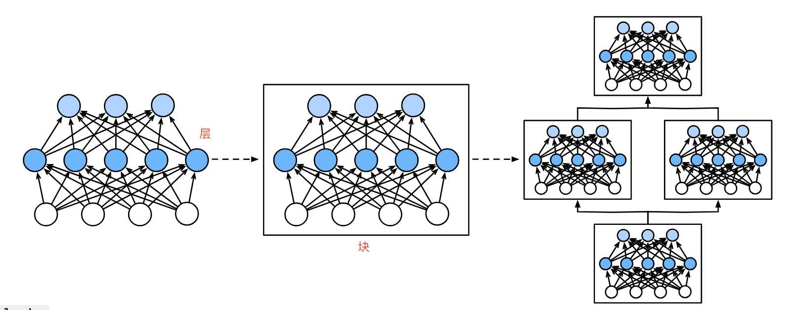
简单来说,如下图,第一个图中间5个神经元组成了一个层。第二图3个层组成了块。第三个图中3个块组成了整个模型。
层
层是神经网络的基本计算单元,负责对输入数据进行特定形式的变换,如线性映射、非线性激活等。其主要的功能是接收输入数据,生成输出结果。其中包含学习参数(如全连接层的权重和偏置)或无参数操作(如激活函数),输出形状可能与输入不同,例如全连接层将维度din映射到dout。
全连接层
layer = nn.Linear(4, 5)  # 输入维度4,输出维度5
X = torch.randn(3, 4)    # 输入形状(3,4)
output = layer(X)        # 输出形状(3,5) :ml-citation{ref="1,3" data="citationList"}
nn.Linerar(4, 5):这里传入两个参数,第一个参数表示输入数据特征维度(示例是4),第二个参数表示输出特征维度(示例是5)。注意这里是特征维度,而不是样本个数,比如这里的特征维度是4,可以输入[2,4],[6,4]即2行4列或6行4列的数据样本。
激活函数层
layer = nn.ReLU()        # 无参数操作
output = layer(torch.tensor([-1, 2, -3]))  # 输出[0, 2, 0] :ml-citation{ref="3,5" data="citationList"}
激活函数层也是单独的一层。激活函数层是神经网络中用于引入非线性的部分,它的作用是帮助网络学习到更加复杂的函数映射。没有激活函数,神经网络只能表示线性函数,而引入非线性后,神经网络可以表示更复杂的模式,从而在各种任务(如分类、回归等)中表现得更好。
自定义层
在神经网络中,自定义层是用户根据具体任务需求自定义实现的层。与内置层(全连接层、卷积层)不同,自定义层可以根据特定的逻辑或行为来扩展模型。它允许你在训练和推理过程中执行特殊的操作或改变标准层的行为。使用自定义层可以使某些模型进行特殊计算,比如自定义正则化、损失函数或特殊的激活函数等。
在pytorch中如何实现自定义层,通常是通过继承torch.nn.Module类来实现的,需要定义的内容如下:
- init:定义层需要的参数或子层。
- forward:定义数据如何通过该层传递并执行相应的计算。
无参数层
无参数层不包含任何需要训练的参数,通常用于执行某些固定的操作或计算。比如激活函数、归一化操作、数学变换等。
import torch
import torch.nn as nn

#继承nn.Module
class custom_relu(nn.Module):
    def __init__(self):
        super().__init__()

    def forward(self, x):
        return torch.maximum(x, torch.tensor(0.0))

layer = custom_relu()
input_data = torch.randn(3, 3)
print(input_data)

output_data = layer(input_data)
print(output_data)
代码运行结果如下:
tensor([[ 0.9986, -0.8549, -0.2031],
        [ 0.8380,  0.6925, -0.9164],
        [ 0.5807, -0.5719,  1.1864]])
tensor([[0.9986, 0.0000, 0.0000],
        [0.8380, 0.6925, 0.0000],
        [0.5807, 0.0000, 1.1864]])
带参数的层
参数层包含可学习的按时,通常执行一些依赖于权重或偏置的计算,比如线性变换、卷积等。参数层通常会在训练过程中优化这些参数。
import torch
import torch.nn as nn

class custom_linear_layer(nn.Module):
    def __init__(self, input_dim, output_dim):
        super().__init__()
        self.weights = nn.Parameter(torch.randn(input_dim, output_dim))
        self.bias = nn.Parameter(torch.randn(output_dim))

    def forward(self, x):
        return torch.matmul(x, self.weights) + self.bias

layer = custom_linear_layer(3, 2)
input_data = torch.randn(5, 3)
print(input_data)
output_data = layer(input_data)
print(output_data)
运行结果如下:
tensor([[-0.7047,  1.8763,  1.8934],
        [-0.1341,  0.4411,  0.2252],
        [ 1.0531,  0.2556, -0.0045],
        [-0.9485,  1.9396, -0.3373],
        [-0.4364,  0.4522, -0.3176]])

tensor([[ 2.2790, -0.5707],
        [ 0.0157, -0.3939],
        [-0.7449, -0.6362],
        [ 0.1973, -1.3335],
        [-0.3929, -0.5201]], grad_fn=<AddBackward0>)
块
块是由多个层组成的复合模块,用于封装重复或复杂功能的代码逻辑,实现模型结构的模块化。包含前向传播逻辑forward的方法、可嵌套其他块或层形成层次化的结构,继承自nn.Module,支持参数管理和自动梯度计算。
Sequential容器
block = nn.Sequential(
    nn.Linear(4, 5),
    nn.ReLU(),
    nn.Linear(5, 3)
)

# 包含3个子层:线性→激活→线性 :ml-citation{ref="6,7" data="citationList"}
Sequential容器用于按顺序定义一个神经网络模块,它将各个子模块按照定义顺序组合在一起,从而实现前向传播。
- 输入:假设输入时一个形状为(batch_size, 4)的张量,表示batch_size个样本,每个样本有4个特征。
- 第一个线性层:输入通过第一个nn.Linear(4, 5), 输出形状变为(batch_size, 5)。
- ReLu激活函数:输出经过第一个nn.ReLU,所有负数变为0,正数保持不变,输出仍为形状(batch_size, 5)。
- 第二个线性层:经过第二个nn.Linear(5, 3),输出形状变为(batch_size, 3)。
import torch
import torch.nn as nn

block = nn.Sequential(
    nn.Linear(4, 5),  # 输入样本是4个特征, 转换为5个特征
    nn.ReLU(),
    nn.Linear(5, 3)) #输出3个特征

input_data = torch.randn(2, 4)
print(input_data)

output_data = block(input_data)
print(output_data)
运行结果:
tensor([[ 0.3054,  1.0160, -1.7137, -0.3744],
        [-0.6882, -0.3049, -1.2769,  0.2835]])
tensor([[ 0.4485,  0.6298, -0.1949],
        [ 0.1992,  0.1609, -0.2480]], grad_fn=<AddmmBackward0>)
自定义块
在pytorch中,自定义块通常是通过继承nn.Module创建的自定义或模型块。可以根据需要组合多个操作或实现一些特定功能,创建属于自己的网络模块。
如何创建自定义块了?
- 基层nn.Module: 需要先继承nn.Module,这是pytorch中所有神经网络模块的基类。
- 定义init方法:在init方法中定义层,例如nn.Linear、nn.Conv2d等操作并初始化他们。
- 定义forward方法:在forward方法中定义输入数据如何通过自定义层进行处理。
import torch
import torch.nn as nn

class custom_block(nn.Module):
    def __init__(self):
        super().__init__()
        self.fc1 = nn.Linear(4, 5)
        self.fc2 = nn.Linear(5, 3)
        self.relu = nn.ReLU()

    def forward(self, x):
        x = self.fc1(x)
        x = self.relu(x)
        x = self.fc2(x)
        return x

custom_block = custom_block()
input_data = torch.randn(2, 4)
print(input_data)
output_data = custom_block(input_data)
print(output_data)
运行结果如下:
tensor([[-0.4663,  0.9429, -0.2072, -1.7672],
        [ 0.6028, -0.2563, -0.3493,  1.2657]])
tensor([[-0.0273, -0.1265, -0.2595],
        [ 0.1276, -0.0837, -0.4265]], grad_fn=<AddmmBackward0>)
复杂块
待补充
参数管理
在深度学习中,参数管理通常指的是如何管理模块中的参数,确保它们在训练过程中得到适当的更新,或者在不同阶段(如训练、验证、测试)进行适当的操作。有效的参数管理有助于提高模型训练的效率和稳定性。
参数访问
import torch
from torch import nn

net = nn.Sequential(
    nn.Linear(4, 8),
    nn.ReLU(),
    nn.Linear(8, 1))

X = torch.rand(size=(2, 4))
y = net(X)
print(y)

print(net[2].state_dict())
print(type(net[2].bias))
print(net[2].bias)
print(net[2].bias.data)
print(net[2].weight.grad)
运行结果如下:
tensor([[-0.1428],
        [-0.1919]], grad_fn=<AddmmBackward0>)

OrderedDict([('weight', tensor([[-0.3178, -0.2009, -0.1120,  0.1502,  0.0054, -0.0864,  0.2142, -0.0564]])), ('bias', tensor([-0.0326]))])  #打印.state_dirct()

<class 'torch.nn.parameter.Parameter'> #-打印.bias
Parameter containing:
tensor([-0.0326], requires_grad=True)

tensor([-0.0326]) #打印.bias.data

None   #打印.weight.grad
也可以使用下面的一次性访问所有参数
print(*[(name, param.shape) for name, param in net[0].named_parameters()])
print(*[(name, param.shape) for name, param in net.named_parameters()])
运行结果:
('weight', torch.Size([8, 4])) ('bias', torch.Size([8]))
('0.weight', torch.Size([8, 4])) ('0.bias', torch.Size([8])) ('2.weight', torch.Size([1, 8])) ('2.bias', torch.Size([1]))
另外可以使用print打印模型的结构
print(net)
运行如下:
Sequential(
  (0): Linear(in_features=4, out_features=8, bias=True)
  (1): ReLU()
  (2): Linear(in_features=8, out_features=1, bias=True)
)
参数初始化
def init_normal(m):
    if type(m) == nn.Linear:
        nn.init.normal_(m.weight, mean=1, std=0.01)
        nn.init.zeros_(m.bias)

net.apply(init_normal)
net[0].weight.data[0], net[0].bias.data[0]
运行结果如下:
(tensor([0.9942, 0.9995, 0.9971, 0.9903]), tensor(0.))
上面的代码定义了一个init_normal函数,改变了weight和bias,初始化为标准差0.01的高斯随机变量且将参数设置为0。
参数绑定
所谓参数绑定,就是将多个层间使用共享参数,下面看示例。
shared = nn.Linear(8, 8)
net = nn.Sequential(nn.Linear(4, 8), nn.ReLU(),
    shared, nn.ReLU(),
    shared, nn.ReLU(),
    nn.Linear(8, 1))

net(X)

print(net)

print(net[2].weight.data[0] == net[4].weight.data[0])
net[2].weight.data[0, 0] = 100
print(net[2].weight.data[0] == net[4].weight.data[0])
运行结果如下:
Sequential(
  (0): Linear(in_features=4, out_features=8, bias=True)
  (1): ReLU()
  (2): Linear(in_features=8, out_features=8, bias=True)
  (3): ReLU()
  (4): Linear(in_features=8, out_features=8, bias=True)
  (5): ReLU()
  (6): Linear(in_features=8, out_features=1, bias=True)
)
tensor([True, True, True, True, True, True, True, True])
tensor([True, True, True, True, True, True, True, True])
可以看到第2层和第4层的参数是一样的,他们不仅值相等,当改变其中一个参数,另一个参数也会一起改变为一样的值。
参数存储
在pytorch中可以调用save和load保存和读取文件,示例如下。
import torch
from torch import nn
from torch.nn import functional as F

x = torch.arange(4)
print(x)
torch.save(x, 'x-file')

x2 = torch.load('x-file')

print(x2)

打印如下:
tensor([0, 1, 2, 3])
tensor([0, 1, 2, 3])
在训练过程中,可以将参数进行保存,下面是示例。
class nlp(nn.Module):
    def __init__(self):
        super().__init__()
        self.hidden = nn.Linear(20, 256)
        self.output = nn.Linear(256, 10)

    def forward(self, x):
        return self.output(F.relu(self.hidden(x)))

net = nlp()
print(net)
X = torch.randn(size=(2, 20))
print(X)
Y = net(X)
print(Y)

torch.save(net.state_dict(), 'nlp.params')


clone = nlp()
clone.load_state_dict(torch.load('nlp.params'))
clone.eval

Y_clone = clone(X)
Y_clone == Y

打印结果:

nlp(
  (hidden): Linear(in_features=20, out_features=256, bias=True)
  (output): Linear(in_features=256, out_features=10, bias=True)
)

tensor([[-1.3927, -1.9475, -0.6044, -0.5835, -0.5661, -0.4240, -1.4481, -0.0627,
          0.7437,  1.0465,  0.1806,  0.1096, -1.2199,  1.1642,  1.0633,  1.3925,
          0.3849,  0.9443, -0.4781,  0.6522],
        [ 1.2506, -0.7369,  0.7148, -0.3734,  1.3801,  0.4163, -1.3707,  0.5407,
         -0.1734, -1.1068, -0.1630,  1.2899,  0.4753,  0.7332,  0.5401, -0.4011,
         -0.5356, -0.5833,  0.8288, -0.5439]])

tensor([[-0.6972, -0.0666,  0.5621, -0.4620, -0.1545,  0.2283,  0.1647,  0.1879,
          0.1907, -0.1658],
        [-0.2174,  0.2586,  0.2867, -0.2213, -0.0090,  0.0687, -0.0382, -0.0477,
         -0.3194,  0.1438]], grad_fn=<AddmmBackward0>)

tensor([[True, True, True, True, True, True, True, True, True, True],
        [True, True, True, True, True, True, True, True, True, True]])
上面的示例中,先调用torch.save(net.state_dirc(), ‘npl.params’)将参数保存起来,然后接着通过load_state_dict(torch.load(‘npl.params’)),将参数读取出来。通过保存参数的方法,可以将训练的实例化进行备份,从上一次保存的参数接着训练。