现代卷积神经网络
深度卷积神经网络AlexNet
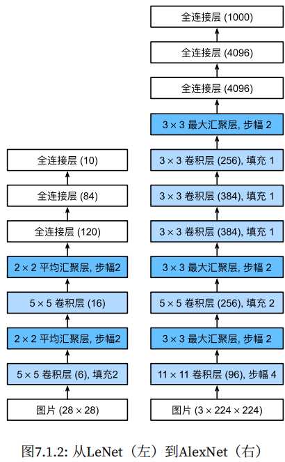
AlexNet相对LeNet的特点就是层数变得更深了,参数变得更多了。AlexNet由八层组成:五个卷积层、两个全连接隐藏层和一个全连接输出层。AlexNet使用ReLU而不是sigmoid作为其激活函数。
import torch
from torch import nn
from d2l import torch as d2l

net = nn.Sequential(
    nn.Conv2d(1, 966, kernel_size=11, stride=4, padding=1), nn.ReLU(),
    nn.MaxPool2d(kernel_size=3, stride=2),
    nn.Conv2d(96, 256, kernel_size=5, padding=2), nn.ReLU(),
    nn.MaxPool2d(kernel_size=3, stride=2),
    nn.Conv2d(256, 384, kernel_size=3, padding=1), nn.ReLU(),
    nn.Conv2d(384, 384, kernel_size=3, padding=1), nn.ReLU(),
    nn.Conv2d(384, 256, kernel_size=3, padding=1), nn.ReLU(),
    nn.MaxPool2d(kernel_size=3, stride=2),
    nn.Flatten(),
    nn.Linear(6400, 4096), nn.ReLU(),
    nn
)

X = torch.randn(1, 1, 224, 224)
for layer in net:
    X=layer(X)
    print(layer.__class__.__name__,'output shape:\t',X.shape)

示例结果:

Conv2d output shape:     torch.Size([1, 96, 54, 54])
ReLU output shape:   torch.Size([1, 96, 54, 54])
MaxPool2d output shape:  torch.Size([1, 96, 26, 26])
Conv2d output shape:     torch.Size([1, 256, 26, 26])
ReLU output shape:   torch.Size([1, 256, 26, 26])
MaxPool2d output shape:  torch.Size([1, 256, 12, 12])
Conv2d output shape:     torch.Size([1, 384, 12, 12])
ReLU output shape:   torch.Size([1, 384, 12, 12])
Conv2d output shape:     torch.Size([1, 384, 12, 12])
ReLU output shape:   torch.Size([1, 384, 12, 12])
Conv2d output shape:     torch.Size([1, 256, 12, 12])
ReLU output shape:   torch.Size([1, 256, 12, 12])
MaxPool2d output shape:  torch.Size([1, 256, 5, 5])
Flatten output shape:    torch.Size([1, 6400])
Linear output shape:     torch.Size([1, 4096])
ReLU output shape:   torch.Size([1, 4096])
Dropout output shape:    torch.Size([1, 4096])
Linear output shape:     torch.Size([1, 4096])
ReLU output shape:   torch.Size([1, 4096])
Dropout output shape:    torch.Size([1, 4096])
Linear output shape:     torch.Size([1, 10])
AlexNet是更大更深的LeNet,比LeNet多了10倍的参数,260倍的计算复杂度。同时添加了丢弃法和ReLU。
使用块的网络VGG
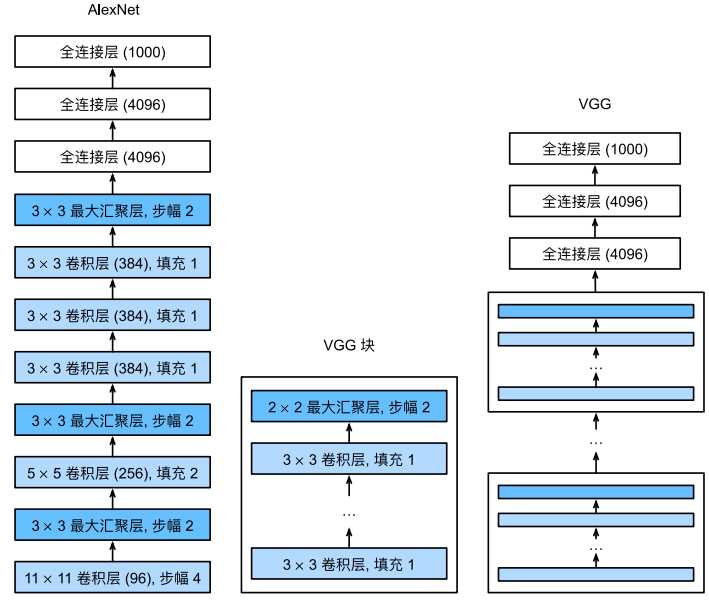
通过AlexNet实践,添加更多的层使得模型的效果更好,但是要添加多少层了?是否有一些通用模版可以提供指导,VGG块就是解决这样的问题。将一些列的卷积层封装为一个块方便调用。
import torch
from torch import nn
from d2l import torch as d2l


def vgg_block(num_convs, in_channels, out_channels):
    layers = []
    for _ in range(num_convs):
        layers.append(nn.Conv2d(in_channels, out_channels,
                                kernel_size=3, padding=1))
        layers.append(nn.ReLU())
        in_channels = out_channels
    layers.append(nn.MaxPool2d(kernel_size=2,stride=2))
    return nn.Sequential(*layers)

def vgg(conv_arch):
    conv_blks = []
    in_channels = 1
    # 卷积层部分
    for (num_convs, out_channels) in conv_arch:
        conv_blks.append(vgg_block(num_convs, in_channels, out_channels))
        in_channels = out_channels

    return nn.Sequential(
        *conv_blks, nn.Flatten(),
        # 全连接层部分
        nn.Linear(out_channels * 7 * 7, 4096), nn.ReLU(), nn.Dropout(0.5),
        nn.Linear(4096, 4096), nn.ReLU(), nn.Dropout(0.5),
        nn.Linear(4096, 10))

conv_arch = ((1, 64), (1, 128), (2, 256), (2, 512), (2, 512))
net = vgg(conv_arch)

X = torch.randn(size=(1, 1, 224, 224))

for blk in net:
    X = blk(X)
    print(blk.__class__.__name__,'output shape:\t',X.shape)

运行结果:
Sequential output shape: torch.Size([1, 64, 112, 112])
Sequential output shape: torch.Size([1, 128, 56, 56])
Sequential output shape: torch.Size([1, 256, 28, 28])
Sequential output shape: torch.Size([1, 512, 14, 14])
Sequential output shape: torch.Size([1, 512, 7, 7])
Flatten output shape: torch.Size([1, 25088])
Linear output shape: torch.Size([1, 4096])
ReLU output shape: torch.Size([1, 4096])
Dropout output shape: torch.Size([1, 4096])
Linear output shape: torch.Size([1, 4096])
ReLU output shape: torch.Size([1, 4096])
Dropout output shape: torch.Size([1, 4096])
Linear output shape: torch.Size([1, 10])
VGG是使用可重复使用的卷积块来构建深度卷积神经网络,不同卷积块的个数和超参数可以得到不同复杂度的变种。
网络中的网络NiN
使用卷积层可以减少训练的参数。但从前面AlexNet或者VGG的示例中,卷积层后面全连接层参数是比较大的
- LeNet: 1655*120 = 48K
- AlexNet: 25655*4096 = 26M
- VGG: 51277*4096 = 102M
哪有没有什么办法可以替换到全连接以减少参数?方法就是将全连接层替换为1*1的卷积层也可以起到全连接层的作用。
import torch
from torch import nn
from d2l import torch as d2l


def nin_block(in_channels, out_channels, kernel_size, strides, padding):
    return nn.Sequential(
        nn.Conv2d(in_channels, out_channels, kernel_size, strides, padding),
        nn.ReLU(),
        nn.Conv2d(out_channels, out_channels, kernel_size=1), nn.ReLU(),
        nn.Conv2d(out_channels, out_channels, kernel_size=1), nn.ReLU())

net = nn.Sequential(
    nin_block(1, 96, kernel_size=11, strides=4, padding=0),
    nn.MaxPool2d(3, stride=2),
    nin_block(96, 256, kernel_size=5, strides=1, padding=2),
    nn.MaxPool2d(3, stride=2),
    nin_block(256, 384, kernel_size=3, strides=1, padding=1),
    nn.MaxPool2d(3, stride=2),
    nn.Dropout(0.5),
    # 标签类别数是10
    nin_block(384, 10, kernel_size=3, strides=1, padding=1),
    nn.AdaptiveAvgPool2d((1, 1)),
    # 将四维的输出转成二维的输出,其形状为(批量大小,10)
    nn.Flatten())

X = torch.rand(size=(1, 1, 224, 224))
for layer in net:
    X = layer(X)
    print(layer.__class__.__name__,'output shape:\t', X.shape)

运行结果:

Sequential output shape:     torch.Size([1, 96, 54, 54])
MaxPool2d output shape:  torch.Size([1, 96, 26, 26])
Sequential output shape:     torch.Size([1, 256, 26, 26])
MaxPool2d output shape:  torch.Size([1, 256, 12, 12])
Sequential output shape:     torch.Size([1, 384, 12, 12])
MaxPool2d output shape:  torch.Size([1, 384, 5, 5])
Dropout output shape:    torch.Size([1, 384, 5, 5])
Sequential output shape:     torch.Size([1, 10, 5, 5])
AdaptiveAvgPool2d output shape:  torch.Size([1, 10, 1, 1])
Flatten output shape:    torch.Size([1, 10])
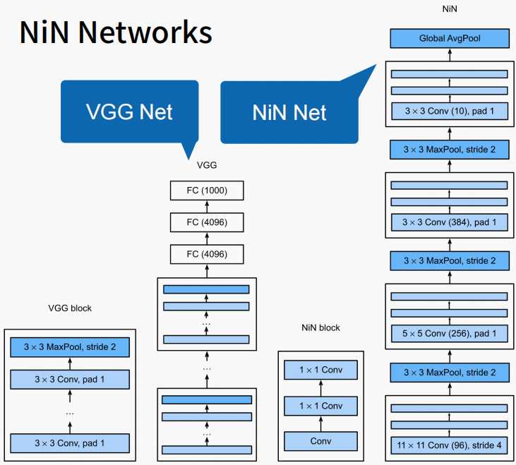
NiN块使用卷积层加两个1*1卷积层,整个架构没有全连接层,降低了参数的数量。
并行连结的网络GoogleNet
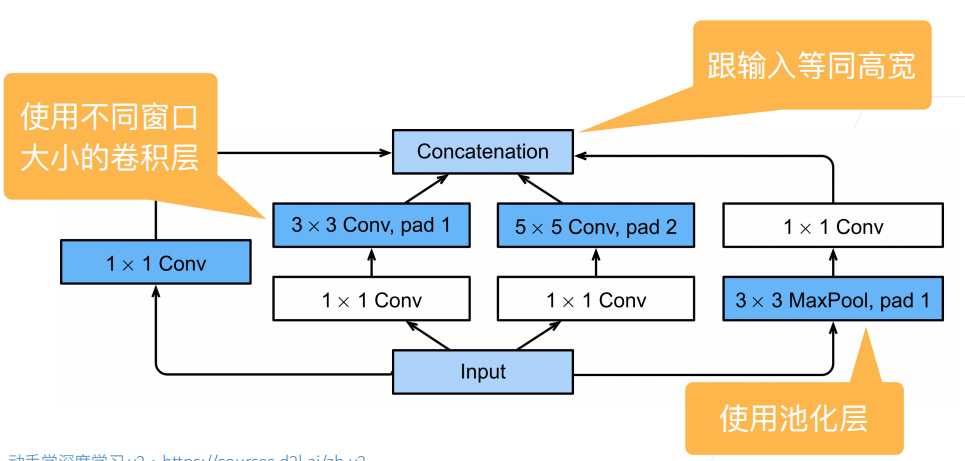
在goodLeNet,基本的卷积块称为Inception块,有四条并行路径组成。googleNet类似于滤波器的组合,可以用各种滤波器尺寸探索图像,不同大小的滤波器可以有效识别不同范围的图像细节。
import torch
from torch import nn
from torch.nn import functional as F
from d2l import torch as d2l


class Inception(nn.Module):
    # c1--c4是每条路径的输出通道数
    def __init__(self, in_channels, c1, c2, c3, c4, **kwargs):
        super(Inception, self).__init__(**kwargs)
        # 线路1,单1x1卷积层
        self.p1_1 = nn.Conv2d(in_channels, c1, kernel_size=1)
        # 线路2,1x1卷积层后接3x3卷积层
        self.p2_1 = nn.Conv2d(in_channels, c2[0], kernel_size=1)
        self.p2_2 = nn.Conv2d(c2[0], c2[1], kernel_size=3, padding=1)
        # 线路3,1x1卷积层后接5x5卷积层
        self.p3_1 = nn.Conv2d(in_channels, c3[0], kernel_size=1)
        self.p3_2 = nn.Conv2d(c3[0], c3[1], kernel_size=5, padding=2)
        # 线路4,3x3最大汇聚层后接1x1卷积层
        self.p4_1 = nn.MaxPool2d(kernel_size=3, stride=1, padding=1)
        self.p4_2 = nn.Conv2d(in_channels, c4, kernel_size=1)

    def forward(self, x):
        p1 = F.relu(self.p1_1(x))
        p2 = F.relu(self.p2_2(F.relu(self.p2_1(x))))
        p3 = F.relu(self.p3_2(F.relu(self.p3_1(x))))
        p4 = F.relu(self.p4_2(self.p4_1(x)))
        # 在通道维度上连结输出
        return torch.cat((p1, p2, p3, p4), dim=1)

b1 = nn.Sequential(nn.Conv2d(1, 64, kernel_size=7, stride=2, padding=3),
                   nn.ReLU(),
                   nn.MaxPool2d(kernel_size=3, stride=2, padding=1))
b2 = nn.Sequential(nn.Conv2d(64, 64, kernel_size=1),
                   nn.ReLU(),
                   nn.Conv2d(64, 192, kernel_size=3, padding=1),
                   nn.ReLU(),
                   nn.MaxPool2d(kernel_size=3, stride=2, padding=1))
b3 = nn.Sequential(Inception(192, 64, (96, 128), (16, 32), 32),
                   Inception(256, 128, (128, 192), (32, 96), 64),
                   nn.MaxPool2d(kernel_size=3, stride=2, padding=1))
b4 = nn.Sequential(Inception(480, 192, (96, 208), (16, 48), 64),
                   Inception(512, 160, (112, 224), (24, 64), 64),
                   Inception(512, 128, (128, 256), (24, 64), 64),
                   Inception(512, 112, (144, 288), (32, 64), 64),
                   Inception(528, 256, (160, 320), (32, 128), 128),
                   nn.MaxPool2d(kernel_size=3, stride=2, padding=1))
b5 = nn.Sequential(Inception(832, 256, (160, 320), (32, 128), 128),
                   Inception(832, 384, (192, 384), (48, 128), 128),
                   nn.AdaptiveAvgPool2d((1,1)),
                   nn.Flatten())

net = nn.Sequential(b1, b2, b3, b4, b5, nn.Linear(1024, 10))
X = torch.rand(size=(1, 1, 96, 96))

for layer in net:
    X = layer(X)
    print(layer.__class__.__name__,'output shape:\t', X.shape)

运行结果:

Sequential output shape:     torch.Size([1, 64, 24, 24])
Sequential output shape:     torch.Size([1, 192, 12, 12])
Sequential output shape:     torch.Size([1, 480, 6, 6])
Sequential output shape:     torch.Size([1, 832, 3, 3])
Sequential output shape:     torch.Size([1, 1024])
Linear output shape:     torch.Size([1, 10])
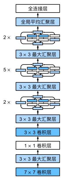
inception块用了4条有不同超参数的卷积层和池化层的路来抽取不同的信息,它主要的优点事模型参数小,计算复杂度第,googleNet用了9个Inception块,是第一个达到上百层的网络。
批量归一化
批量归一化(Batch Normalization,简称BN)是一种在训练神经网络时用于加速收敛、提高模型稳定性和提高性能的技术。它通过规范化每一层的输入,确保每一层的输入具有相同的分布,从而减少了不同层之间数据分布的变化,避免了梯度消失或爆炸问题。
具体来说,批量归一化的过程如下:
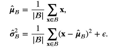
- 计算均值和方差:对于每一层的输入,计算该层在一个小批量(batch)上的均值和方差。通常是在训练过程中,对每个特征(特征是指每一维数据)独立地计算均值和方差。
-
归一化:利用上述计算出的均值和方差,对输入数据进行归一化。每个输入的值减去该批量的均值并除以该批量的标准差,从而将输入的分布调整为均值为0,方差为1的标准正态分布。
-
缩放与偏移:归一化后的数据会通过一个可学习的参数进行缩放(scale)和偏移(shift),即引入两个新的参数:γ(gamma)和β(beta)。这些参数允许模型恢复某些可能丢失的信息。
简单理解批量归一化就是对输入的数据按照按照小批量的均值、方差、\boldsymbol{\gamma}和\boldsymbol{\beta}的公式进行处理,得到输出后的数据。这样也相当于对输入的数据加入了噪音,因此不要和丢弃法混合使用。
\mathrm{BN}(\mathbf{x}) = \boldsymbol{\gamma} \odot \frac{\mathbf{x} – \hat{\boldsymbol{\mu}}_\mathcal{B}}{\hat{\boldsymbol{\sigma}}_\mathcal{B}} + \boldsymbol{\beta}.
- $\hat{\boldsymbol{\mu}}_\mathcal{B}$:是小批量 $\mathcal{B}$的样本均值
- $\hat{\boldsymbol{\sigma}}_\mathcal{B}$:是小批量$\mathcal{B}$的样本标准差。
由于单位方差(与其他一些魔法数)是一个主观的选择,因此我们通常包含拉伸参数(scale)\boldsymbol{\gamma}和偏移参数(shift)\boldsymbol{\beta},它们的形状与\mathbf{x}相同。需要注意的是,\boldsymbol{\gamma}和\boldsymbol{\beta}是需要与其他模型参数一起学习的参数。
由于在训练过程中,中间层的变化幅度不能过于剧烈,而批量规范化将每一层主动居中,并将它们重新调整为给定的平均值和大小。
如下所示:
net = nn.Sequential(
    nn.Conv2d(1, 6, kernel_size=5), BatchNorm(6, num_dims=4), nn.Sigmoid(),
    nn.AvgPool2d(kernel_size=2, stride=2),
    nn.Conv2d(6, 16, kernel_size=5), BatchNorm(16, num_dims=4), nn.Sigmoid(),
    nn.AvgPool2d(kernel_size=2, stride=2), nn.Flatten(),
    nn.Linear(16*4*4, 120), BatchNorm(120, num_dims=2), nn.Sigmoid(),
    nn.Linear(120, 84), BatchNorm(84, num_dims=2), nn.Sigmoid(),
    nn.Linear(84, 10))
上面的示例中,在卷积层的后面使用了BatchNorm(6, num_dims=4)批量归一化。批量归一化就是固定小批量中的均值和方差,然后学习出适合的偏移和缩放,这样可以加速手链速度,但一般不改变模型的精度
残差网络ResNet
使用残差可以使得模型可以容易得叠加很多层,先来看看,什么是残差网络?残差网络就是由一系列的残差块组成,下图就是一个残差块。用公式表示就是:X_{l+1} = X_l + F(X_l, W_l),,其中F(X_l, W_l)是残差。
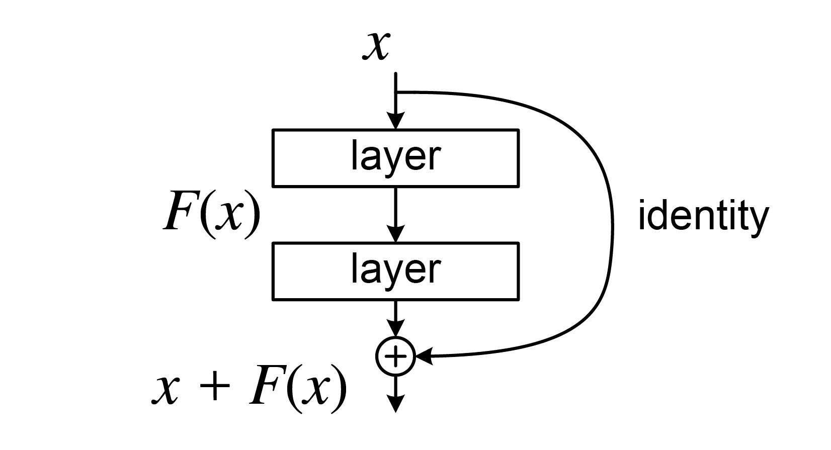
残差块分有直接映射+残差两部分组成,表示输入经过残差块或直接映射到底输出。
在传统的神经网络中,输入X会经过多层变换(如卷积、激活等),最终得出输出Y。这些变换会逐渐改变输入的信息,试图将其转化为输出的目标形式。而在残差网络中,模型不仅学习输入X到输出 Y的映射,而是学习输入和输出之间的差异,即残差。数学上,可以表示为:
Y’ = X + F(X)
其中,Y’是网络的最终输出,F(X) 是通过多个层(如卷积层、激活层等)处理后的结果(这个部分是“残差”),而 X是输入。这里,F(X) 就是输入 X与输出Y之间的差异。也就是说X加上一个什么样的函数,能逼近Y。
为什么学习残差更容易?
学习从输入到输出的直接映射可能很复杂,特别是在深层网络中,因为输入经过多次变换后,最终的输出可能与输入有很大的差异。传统网络需要学习整个映射过程,这样可能导致训练时出现梯度消失或信息丢失的问题。但是,学习输入和输出之间的残差通常更简单。因为,通常情况下,输入和输出之间的差异(残差)可能是一个相对较小且较简单的函数。这使得网络能更容易捕捉到输入与输出之间的“偏差”,而不是直接学习整个变换过程。
举个例子
假设我们有一个非常深的网络,输入 X 和目标输出 Y 之间的关系很复杂。传统的网络可能需要直接学习一个非常复杂的映射函数。与此不同,残差网络并不直接学习这个复杂的映射,而是学习输入 X 和输出 Y 之间的差异。
例如,如果输出 Y 只是输入 X 加上一个小的偏差(例如,Y = X + \epsilon),那么残差 F(X) = \epsilon 就是一个简单的学习目标。这个“差异”往往比直接学习整个映射来得容易。
可以把残差看作是一个补充信息。例如,假设你有一个图片分类任务,输入是图片,输出是类别标签。传统网络要直接将图片映射到标签,这个过程非常复杂。而在残差网络中,网络实际上在学习的是“这张图片与类别标签之间的差异”。如果输入与输出之间的关系可以通过一个小的差异来描述,那么网络只需要学习这个差异,训练起来会更容易。
残差网络的关键在于它将学习的重点从直接映射 X \to Y 转变为学习输入和输出之间的差异(残差) F(X)。这样,网络不仅能更加高效地训练,还能避免深层网络中常见的梯度消失和信息衰减问题。
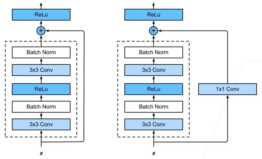
上图有两个残差块,左图中X可以直接到输出,右图中X经过1*1 Conv层到输出。对于左图当虚线框中的块如果是0,那么X还是原来的X。通过残差在在计算梯度时,可以使得接近输入层的参数可以得到更好的训练,因为经过多层神经网络后,最后一层可以通过“捷径”直到前面的层,这样梯度计算就更方便。
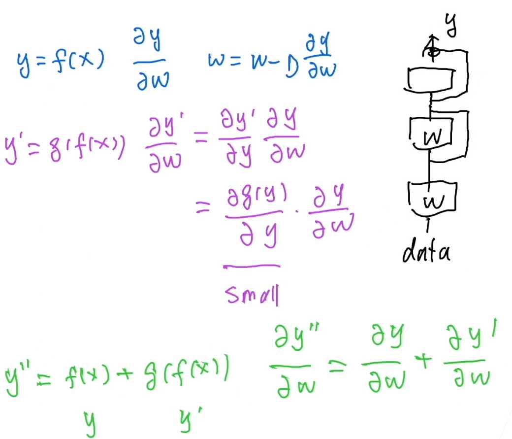
使用残差可以高效的训练靠近输入的神经网络的参数,避免层数的加深,越靠近输入的神经网络层参数变化较小而导致难以训练,因为梯度的计算是从后往前,而最后的参数如果相对较小时,通过链式法则计算(相乘)的前面梯度会更小,也就是前面层数w变化就小。
import torch
from torch import nn
from torch.nn import functional as F
from d2l import torch as d2l
class Residual(nn.Module): #@save
def __init__(self, input_channels, num_channels,
use_1x1conv=False, strides=1):
super().__init__()
self.conv1 = nn.Conv2d(input_channels, num_channels,
kernel_size=3, padding=1, stride=strides)
self.conv2 = nn.Conv2d(num_channels, num_channels,
kernel_size=3, padding=1)
if use_1x1conv:
self.conv3 = nn.Conv2d(input_channels, num_channels,
kernel_size=1, stride=strides)
else:
self.conv3 = None
self.bn1 = nn.BatchNorm2d(num_channels)
self.bn2 = nn.BatchNorm2d(num_channels)
def forward(self, X):
Y = F.relu(self.bn1(self.conv1(X)))
Y = self.bn2(self.conv2(Y))
if self.conv3:
X = self.conv3(X)
Y += X #---------------->核心算法
return F.relu(Y)
#构建一个残差块
def resnet_block(input_channels, num_channels, num_residuals,
first_block=False):
blk = []
for i in range(num_residuals):
if i == 0 and not first_block:
blk.append(Residual(input_channels, num_channels,
use_1x1conv=True, strides=2))
else:
blk.append(Residual(num_channels, num_channels))
return blk
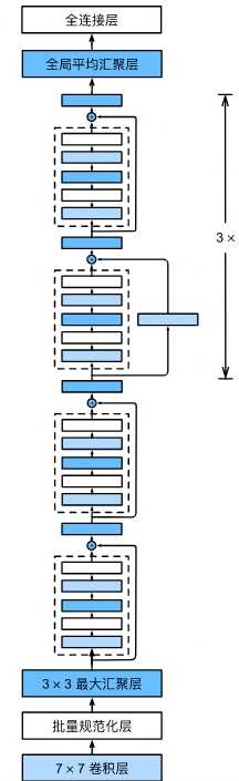
b1 = nn.Sequential(nn.Conv2d(1, 64, kernel_size=7, stride=2, padding=3),
nn.BatchNorm2d(64), nn.ReLU(),
nn.MaxPool2d(kernel_size=3, stride=2, padding=1))
#b2~b5是残差块生成
b2 = nn.Sequential(*resnet_block(64, 64, 2, first_block=True))
b3 = nn.Sequential(*resnet_block(64, 128, 2))
b4 = nn.Sequential(*resnet_block(128, 256, 2))
b5 = nn.Sequential(*resnet_block(256, 512, 2))
net = nn.Sequential(b1, b2, b3, b4, b5,
nn.AdaptiveAvgPool2d((1,1)),
nn.Flatten(), nn.Linear(512, 10))
X = torch.rand(size=(1, 1, 224, 224))
for layer in net:
X = layer(X)
print(layer.__class__.__name__,'output shape:\t', X.shape)
运行结果:
Sequential output shape: torch.Size([1, 64, 56, 56])
Sequential output shape: torch.Size([1, 64, 56, 56])
Sequential output shape: torch.Size([1, 128, 28, 28])
Sequential output shape: torch.Size([1, 256, 14, 14])
Sequential output shape: torch.Size([1, 512, 7, 7])
AdaptiveAvgPool2d output shape: torch.Size([1, 512, 1, 1])
Flatten output shape: torch.Size([1, 512])
Linear output shape: torch.Size([1, 10])
Sequential(
  (0): Sequential(
    (0): Conv2d(1, 64, kernel_size=(7, 7), stride=(2, 2), padding=(3, 3))
    (1): BatchNorm2d(64, eps=1e-05, momentum=0.1, affine=True, track_running_stats=True)
    (2): ReLU()
    (3): MaxPool2d(kernel_size=3, stride=2, padding=1, dilation=1, ceil_mode=False)
  )
  (1): Sequential(
    (0): Residual(
      (conv1): Conv2d(64, 64, kernel_size=(3, 3), stride=(1, 1), padding=(1, 1))
      (conv2): Conv2d(64, 64, kernel_size=(3, 3), stride=(1, 1), padding=(1, 1))
      (bn1): BatchNorm2d(64, eps=1e-05, momentum=0.1, affine=True, track_running_stats=True)
      (bn2): BatchNorm2d(64, eps=1e-05, momentum=0.1, affine=True, track_running_stats=True)
    )
    (1): Residual(
      (conv1): Conv2d(64, 64, kernel_size=(3, 3), stride=(1, 1), padding=(1, 1))
      (conv2): Conv2d(64, 64, kernel_size=(3, 3), stride=(1, 1), padding=(1, 1))
      (bn1): BatchNorm2d(64, eps=1e-05, momentum=0.1, affine=True, track_running_stats=True)
      (bn2): BatchNorm2d(64, eps=1e-05, momentum=0.1, affine=True, track_running_stats=True)
    )
  )
  (2): Sequential(
    (0): Residual(
      (conv1): Conv2d(64, 128, kernel_size=(3, 3), stride=(2, 2), padding=(1, 1))
      (conv2): Conv2d(128, 128, kernel_size=(3, 3), stride=(1, 1), padding=(1, 1))
      (conv3): Conv2d(64, 128, kernel_size=(1, 1), stride=(2, 2))
      (bn1): BatchNorm2d(128, eps=1e-05, momentum=0.1, affine=True, track_running_stats=True)
      (bn2): BatchNorm2d(128, eps=1e-05, momentum=0.1, affine=True, track_running_stats=True)
    )
    (1): Residual(
      (conv1): Conv2d(128, 128, kernel_size=(3, 3), stride=(1, 1), padding=(1, 1))
      (conv2): Conv2d(128, 128, kernel_size=(3, 3), stride=(1, 1), padding=(1, 1))
      (bn1): BatchNorm2d(128, eps=1e-05, momentum=0.1, affine=True, track_running_stats=True)
      (bn2): BatchNorm2d(128, eps=1e-05, momentum=0.1, affine=True, track_running_stats=True)
    )
  )
  (3): Sequential(
    (0): Residual(
      (conv1): Conv2d(128, 256, kernel_size=(3, 3), stride=(2, 2), padding=(1, 1))
      (conv2): Conv2d(256, 256, kernel_size=(3, 3), stride=(1, 1), padding=(1, 1))
      (conv3): Conv2d(128, 256, kernel_size=(1, 1), stride=(2, 2))
      (bn1): BatchNorm2d(256, eps=1e-05, momentum=0.1, affine=True, track_running_stats=True)
      (bn2): BatchNorm2d(256, eps=1e-05, momentum=0.1, affine=True, track_running_stats=True)
    )
    (1): Residual(
      (conv1): Conv2d(256, 256, kernel_size=(3, 3), stride=(1, 1), padding=(1, 1))
      (conv2): Conv2d(256, 256, kernel_size=(3, 3), stride=(1, 1), padding=(1, 1))
      (bn1): BatchNorm2d(256, eps=1e-05, momentum=0.1, affine=True, track_running_stats=True)
      (bn2): BatchNorm2d(256, eps=1e-05, momentum=0.1, affine=True, track_running_stats=True)
    )
  )
  (4): Sequential(
    (0): Residual(
      (conv1): Conv2d(256, 512, kernel_size=(3, 3), stride=(2, 2), padding=(1, 1))
      (conv2): Conv2d(512, 512, kernel_size=(3, 3), stride=(1, 1), padding=(1, 1))
      (conv3): Conv2d(256, 512, kernel_size=(1, 1), stride=(2, 2))
      (bn1): BatchNorm2d(512, eps=1e-05, momentum=0.1, affine=True, track_running_stats=True)
      (bn2): BatchNorm2d(512, eps=1e-05, momentum=0.1, affine=True, track_running_stats=True)
    )
    (1): Residual(
      (conv1): Conv2d(512, 512, kernel_size=(3, 3), stride=(1, 1), padding=(1, 1))
      (conv2): Conv2d(512, 512, kernel_size=(3, 3), stride=(1, 1), padding=(1, 1))
      (bn1): BatchNorm2d(512, eps=1e-05, momentum=0.1, affine=True, track_running_stats=True)
      (bn2): BatchNorm2d(512, eps=1e-05, momentum=0.1, affine=True, track_running_stats=True)
    )
  )
  (5): AdaptiveAvgPool2d(output_size=(1, 1))
  (6): Flatten(start_dim=1, end_dim=-1)
  (7): Linear(in_features=512, out_features=10, bias=True)
)